Dual space (linear algebra)

From Knowino

Jump to: navigation, search

In linear algebra, the dual V^∗ of a finite-dimensional vector space V is the vector space of linear functionals (also known as one-forms) on V. Both spaces, V and V^∗, have the same dimension. If V is equipped with an inner product, V and V^∗ are naturally isomorphic, which means that there exists a one-to-one correspondence between the two spaces that is defined without use of bases. (This isomorphism does not generally exist for infinite-dimensional inner product spaces).

The importance of a dual vector space arises in tensor calculus from the fact that elements of V and of V^∗ transform contragrediently. One expresses this by stating that mixed tensors have contravariant components in the dual space V^∗ and covariant components in the original space V. Covariant and contravariant components can be contracted to tensors of lower rank.

In crystallography and solid state physics the dual space of ℝ³ is often referred to as reciprocal space.

[edit] Definition

First an arbitrary finite-dimensional vector space V over the field ℝ of real numbers is considered that is not necessarily equipped with a norm or inner product. The dual linear space V^∗ of V is distinct from V. The linear space V^∗ consisting of linear functionals on V, the latter are introduced first.

A functional α on V is the map

$\alpha: \quad V \rightarrow \mathbb{R} \quad\hbox{with}\quad \langle \alpha \mid v\rangle \in \mathbb{R},\quad v \in V.$

The functional α is linear if

$\langle \alpha\mid c v + c' v'\rangle = c \langle \alpha \mid v\rangle + c' \langle \alpha \mid v'\rangle, \quad v,\;v' \in V, \quad c,\;c' \in \mathbb{R}.$

From linearity follows that any α maps the zero element of V onto the number 0∈ℝ.

If distributivity is postulated, the space V^∗ of linear functionals is a vector space; that is, with α and α′ also cα + c′α′ is a linear functional,

$\langle c\;\alpha + c'\;\alpha' \mid v \rangle = c \langle\alpha\mid v\rangle + c' \langle\alpha'\mid v\rangle \in \mathbb{R}, \quad \alpha,\;\alpha' \in V^\ast.$

The zero vector of V^∗ is the linear functional that maps every element of V onto 0 ∈ ℝ; this zero functional is written as ω.

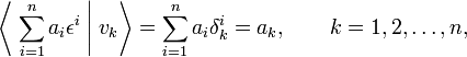
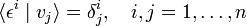
The dimensions of a vector space and its dual are equal. In order to show this, we let v₁, v₂,..., v_n be a basis of V. Any element of V can be uniquely expanded in terms of these n basis elements. Further, when the effect of an arbitrary linear functional α ∈ V^∗ on the n basis elements of V is given, the effect of α on any element of V is determined uniquely; this follows from the linearity of α. Consider now the n linear functionals ε^j defined by

$\langle \epsilon^j \mid v_i \rangle = \delta^j_{i},\quad i,j=1,2, \ldots, n.$

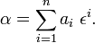
where δ^j_i is the Kronecker delta (unity if i = j, 0 otherwise). Any linear functional can be expressed as a linear combination of the ε^j. Indeed, let an arbitrary linear functional α be given by

$\langle \alpha \mid v_k\rangle = a_k \in \mathbb{R},\quad k=1,2, \dots, n.$

The functional

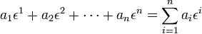
$a_1 \epsilon^1 + a_2 \epsilon^2 + \cdots + a_n \epsilon^n = \sum_{i=1}^n a_i \epsilon^i$

gives obviously the same effect as α on the basis

$\left\langle\; \sum_{i=1}^n a_i \epsilon^i\; \Bigg\vert\; v_k \right\rangle = \sum_{i=1}^n a_i \delta^i_{k} = a_k,\qquad k=1,2, \ldots, n,$

so that the arbitrary linear functional α is equal to the linear combination

$\alpha = \sum_{i=1}^n a_i \;\epsilon^i.$

Further the ε^j are linearly independent. That is, if

$\omega = c_1\epsilon^1 + c_2\epsilon^2+ \cdots c_k\epsilon^k+\cdots + c_n\epsilon^n$

then c_k = 0 for all k=1, ...,n. Consider the coefficient c_k (k arbitrary with 1≤ k ≤ n) and

$0 = \langle \omega \mid v_k\rangle = \langle c_1\epsilon^1 + c_2\epsilon^2+ \cdots c_k\epsilon^k+\cdots + c_n\epsilon^n\mid v_k\rangle = c_k.$

Hence in the expansion of the zero vector ω all expansion coefficients are zero, and it follows that the elements {ε^j | j=1,2,..., n} are linearly independent. Therefore, the ε^j are a basis of V^∗ and dim V^∗ = dim V = n.

One calls the bases v₁, v₂, ..., v_n and ε¹, ε², ..., εⁿ with

$\langle \epsilon^i \mid v_j \rangle = \delta^i_j,\quad i,j=1,\ldots,n$

biorthogonal (or sometimes dual).

[edit] The dual of the dual

Since the linear space V above was arbitrary, the dual of any finite-dimensional linear space may be defined. A legitimate question is: what is the dual of V^∗? The answer is: V. In order to see this, we interpret v ∈ V as a mapping of α onto an element of ℝ,

$v:\quad V^{\ast} \rightarrow \mathbb{R}\quad\hbox{with}\quad v:\; \alpha \rightarrow \langle \alpha \mid v \rangle \in \mathbb{R}.$

As a mapping v acts to the left in the braket ⟨..|..⟩. If so wished, one could let act v to the right by defining

⟨ v | α⟩ := ⟨ α | v ⟩,

but this definition is not necessary and will not be introduced. In any case v is a functional on V^∗. It is a linear functional because (v acts to the left),

$\langle c\;\alpha + c'\;\alpha' \mid v \rangle = c \langle\alpha\mid v\rangle + c' \langle\alpha'\mid v\rangle \in \mathbb{R}, \quad \alpha,\;\alpha' \in V^\ast.$

The domain of v is all of V^∗, because by definition V^∗ contains all linear functionals on V. If there is a linear functional β such that ⟨ β | v ⟩ ∈ ℝ, the functional β is by definition in V^∗ and the action of v on β is defined, i.e., β is in the domain of v. Conversely, suppose that x is an arbitrary linear functional on V^∗ with

$x:\quad \epsilon^i \mapsto \xi_i \in \mathbb{R},\quad i=1,2,\ldots,n.$

Consider the element x′ ∈ V with the components ξ_i

$x' = \sum_{j=1}^n v_j \; \xi_j .$

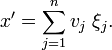
Because of distributivity, the functional x′ maps the basis of V^∗thus,

$x':\quad \epsilon^i \rightarrow \langle \epsilon^i \mid x'\rangle = \sum_{j=1}^n \langle \epsilon^i \mid v_j\rangle \; \xi_j = \xi_i,\qquad i=1,2,\ldots,n.$

Hence x′ = x, and it follows that V contains all linear functionals on V^∗. Conclusion: V^∗∗ (the space of all linear functionals on V^∗) is equal to V. The pair

$\langle\alpha \mid v \rangle \in \mathbb{R}$

is symmetric: α (∈ V^∗) maps v and v (∈ V and ∈ V^∗∗) maps α onto the same real number. It is emphasized that the natural isomorphism between V and V^∗∗ is defined without need for an inner product or basis on V.

[edit] Dual transformations

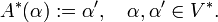
Let A be an arbitrary endomorphism of V (linear map V → V). Let α ∈ V^∗ and let α′ be the linear functional,

$\langle \alpha' \mid v \rangle = \langle \alpha \mid A(v) \rangle, \quad \forall v \in V.$

Define the dual transformation A^∗: V^∗ → V^∗ of A by

$A^{\ast}(\alpha) := \alpha', \quad \alpha, \alpha' \in V^{\ast}.$

It is easy to show that A^∗ is linear. Indeed,

$\begin{align} \langle c_1 \alpha_1 + c_2\alpha_2 \mid A(v) \rangle &= \langle A^{\ast}(c_1 \alpha_1 + c_2\alpha_2) \mid v\rangle \\ &= c_1 \langle \alpha_1 \mid A(v) \rangle + c_2\langle \alpha_2 \mid A(v) \rangle = c_1 \langle A^{\ast}(\alpha_1) \mid v \rangle + c_2 \langle A^{\ast}(\alpha_2) \mid v \rangle \end{align}$

and since this holds for all v it can be concluded that

$A^{\ast}(c_1 \alpha_1 + c_2\alpha_2) = c_1 A^{\ast}(\alpha_1) + c_2 A^{\ast}(\alpha_2),$

so that A^∗ is linear (is an endomorphism of V^∗). A mnemonic is: the transformation A^∗ is defined by the "turnover rule":

$\langle A^{\ast}(\alpha) \mid v \rangle = \langle \alpha \mid A(v) \rangle, \quad \forall v \in V.$

The dual of the identity E on V is the identity on V^∗; the zero map on V has as dual the zero map on V^∗. Let A and B be linear maps of V into itself, then

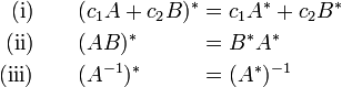
$\begin{alignat}{2} \text{(i)} & \qquad (c_1 A + c_2 B)^{\ast} &&= c_1 A^{\ast} + c_2 B^{\ast} \\ \text{(ii)} & \qquad (A B)^{\ast} &&= B^{\ast} A^{\ast} \\ \text{(iii)}& \qquad (A^{-1})^\ast &&= (A^{\ast})^{-1} \\ \end{alignat}$

Property (i) is self-evident. Property(ii) follows thus,

$\langle \alpha \mid (AB)(v)\; \rangle = \langle \alpha \mid A \big(B(v)\big)\; \rangle = \langle A^{\ast}(\alpha) \mid B(v)\; \rangle = \langle B^{\ast}\big( A^{\ast}(\alpha)\big) \mid v \rangle = \langle (AB)^{\ast}(\alpha) \mid v \rangle$

which is true for any v and α. Property (iii) is only valid if the inverse A⁻¹ exists, it then states that the inverse of the dual also exists. This property follows immediately from (ii) (take B = A⁻¹) and the fact that the dual of the identity on V is the identity on V^∗.

[edit] Matrices

The transformations A and A^∗ being linear, they are each in 1-1 correspondence with a matrix, once a basis of the respective space has been chosen. Write:

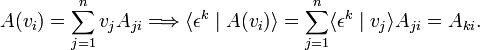
$A(v_i) = \sum_{j=1}^n v_j A_{ji} \Longrightarrow \langle \epsilon^k \mid A(v_i) \rangle = \sum_{j=1}^n \langle \epsilon^k \mid v_j \rangle A_{ji} = A_{ki}.$

On the other hand,

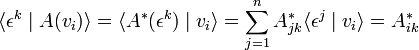
$\langle \epsilon^k \mid A(v_i) \rangle = \langle A^{\ast}(\epsilon^k) \mid v_i \rangle = \sum_{j=1}^n A^{\ast}_{jk} \langle \epsilon^j \mid v_i \rangle = A^{\ast}_{ik}$

so that

$A_{ki} = A^{\ast}_{ik} \Longrightarrow \mathbf{A}^{\mathrm{T}} = \mathbf{A}^{\ast},$

where the superscript T stands for matrix transposition. The matrix of A^∗ is equal to the transpose of the matrix of A.

[edit] Basis transformation

If one transforms simultaneously biorthogonal bases of V and V^∗ to new bases that are again biorthogonal, the matrices effecting the transformation are contragredient to each other (transpose and inverse).

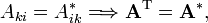
Write, in order to show this, the new bases in terms of the old for V and V^∗, respectively,

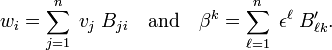
$w_i = \sum_{j=1}^n\; v_j \;B_{ji} \quad\hbox{and}\quad \beta^k = \sum_{\ell=1}^n\; \epsilon^\ell \;B'_{\ell k} .$

The matrices B and B′ are invertible (they map bases onto bases). The new and the old bases are biorthogonal

$\delta^k_i = \langle \beta^k \mid w_i \rangle = \sum_{j,\ell =1 }^n B_{ji}B'_{\ell k} \langle \epsilon^\ell \mid v_j \rangle = \sum_{j,\ell =1 }^n B_{ji}B'_{\ell k} \delta^\ell_j = \sum_{j=1 }^n B_{ji}B'_{j k}.$

As matrices:

$\mathbf{B}^\mathrm{T} \mathbf{B'} = \mathbf{I},$

where I is the n×n identity matrix with general element δ^k_i. In conclusion,

$\mathbf{B'} = \left(\mathbf{B^{-1}}\right)^{\mathrm{T}}.$

[edit] Inner product spaces

Let an inner product (v, w) on V be given. The inner product is the bilinear function on the Cartesian product:

$V\times V \rightarrow \mathbb{R} \quad \hbox{with}\quad v,w \mapsto (v,w) \in \mathbb{R}.$

It is assumed that the inner product is symmetric: (v, w) = (w, v) and non-degenerate: (w, v) = 0 for all w ∈ V if and only if v = 0. It is not assumed that the inner product is definite, i.e., it is possible that (v, v) = 0 while v ≠ 0.

The natural (independent of basis) linear map χ: V → V^∗ defined for a given v ∈ V by:

$\langle \chi(v) \mid w \rangle := (v,\;w), \quad \forall w \in V,$

is a vector space isomorphism between V and V^∗. In the first place, as was shown earlier, dim V = dim V^∗. Secondly χ is invertible. Namely, suppose that v belongs to the kernel of the linear map χ, that is, χ(v) = ω, the null functional. Then

$\langle \chi(v) | w \rangle = (v,\; w) = \langle \omega | w \rangle = 0, \quad \forall w\in V.$

From the non-degeneracy of the inner product it follows that v = 0: the kernel of χ contains only the zero vector. So, χ is one-to-one with a domain and range that cover the respective spaces, and thus χ is a vector space isomorphism. Since χ is defined without bases, the two spaces are naturally isomorphic. In conclusion: it is possible to identify V^∗ with V when V has a non-degenerate inner product.

An example of such identification is the vector product a×b of two vectors in ℝ³. One can define this product as proportional to the wedge product (antisymmetric tensor) $\mathbf{a}\wedge\mathbf{b}$ , and the space of wedge products as a dual space of ℝ³ (see the example below). More commonly one considers the vector product a×b as an element of ℝ³—one thus identifies $\mathbb{R}^3\wedge\mathbb{R}^3$ with ℝ³.

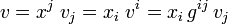
A biorthogonal (dual) basis may be defined within the space V. An upper/lower (also known as contravariant/covariant) index notation is convenient together with the Einstein summation convention^[1] that states that a summation is implied when in a product the same index appears twice. The metric (or fundamental) tensor g is needed,

$g_{ij} := (v_i, v_j), \quad i,j=1,2, \ldots, n,$

where {v_i } is a basis of V. Because the inner product is symmetric and non-degenerate, the tensor g is symmetric and invertible.^[2] Introduce a notation for the inverse of g,

$g^{ij} := (g^{-1})_{ij}\quad \Longleftrightarrow \quad g^{ij} g_{jk} = \delta^{i}_{k},$

where δⁱ_k is the Kronecker delta. (The use of upper indices on g⁻¹ and vectors implies contravariance of these indices; this is indeed the case, see tensor). Define now a biorthogonal basis of V by raising indices of the basis elements v_i, and recall that g is non-singular, so that the set {v^j} is linearly independent of dimension n and accordingly a basis of V,

$v^j := v_i \; g^{ij}\quad\hbox{with}\quad (v^j, v_k) = (v_i, v_k) g^{ij} = g_{ik} g^{ij} = g_{ki} g^{ij} =\delta^{j}_{k}.$

Writing the basis of V^∗ biorthogonal to {v_i } as {ε^j } and comparing the following two expressions

$\langle \epsilon^j \mid v_k \rangle = \delta^j_k \quad\hbox{and}\quad (v^j,v_k) = \delta^{j}_{k}$

one sees a close correspondence between the two bases biorthogonal to { v_k }. The bases belong to different spaces, but because they are so closely connected, it is often stated that "linear combinations of the basis { vⁱ } belong to the dual of V." Strictly speaking one should include the isomorphism χ: vⁱ → εⁱ, but the appearance of χ obscures the notation and is therefore omitted. Conversely, when it is stated that x_i εⁱ belongs to V one should make the (mental) substitution εⁱ → vⁱ in this expression.

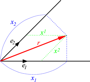
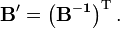
Example: vector r (red) in ℝ². Space is spanned by non-orthogonal unit vectors e₁ and e₂.
r = x¹e₁ + x²e₂ (green).
x₁ = e₁⋅r and x₂ = e₂⋅r (blue).

If one writes

$v = x^j\; v_j = x_i\; v^i = x_i\, g^{ij}\, v_j$

then it follows that

$x^j = x_i\, g^{ij} \quad\Longleftrightarrow\quad x_j = x^i\, g_{ij}$

which shows that the inverse g⁻¹ of the fundamental (metric) tensor transforms the covariant component x_i into the contravariant component x^j (raises the index) of the same vector v ∈ V, and vice versa: g lowers the index of a vector component.

[edit] Example

In a small change of notation, one may write

$\mathbf{r} = x^i\;\mathbf{e}_i \Longrightarrow \mathbf{e}_j \cdot \mathbf{r} = x^i \mathbf{e}_j \cdot \mathbf{e}_i = g_{ji} x^i = x_j,$

where {e_k } is a non-orthogonal basis of V, the centered dot stands for an inner product and r ∈ V. The relation between the contravariant components x^k and the contravariant components x_k are shown in the figure for V = ℝ².

[edit] Application: reciprocal space

Let us consider V = ℝ³ with the usual positive definite inner product written as a centered dot

$\mathbf{a}\cdot\mathbf{b} \equiv (\mathbf{a},\;\mathbf{b}), \quad \mathbf{a},\;\mathbf{b} \in \mathbb{R}^3.$

The triple product plays an important role

$[ \mathbf{a}\;\mathbf{b}\;\mathbf{c}] := (\mathbf{a}\times\mathbf{b})\cdot\mathbf{c}$

where the × stand for a vector product. The quantity between square brackets is a determinant (a three-fold wedge product). The determinant vanishes in case of linear dependence

$[ \mathbf{a}\;\mathbf{b}\;\mathbf{c}] = 0 \quad\Longleftrightarrow\quad\hbox{if}\; \{\mathbf{a},\;\mathbf{b},\;\mathbf{c} \} \;\;\hbox{linearly dependent}.$

In particular, the determinant vanishes if a vector appears at least twice in the determinant.

Consider a non-orthogonal, non-normalized basis a₁, a₂, a₃ of ℝ³. Define vectors

$\begin{align} \mathbf{a}^1 &:= \frac{\mathbf{a}_2\times\mathbf{a}_3}{[ \mathbf{a}_1\;\mathbf{a}_2\;\mathbf{a}_3]} \\ \mathbf{a}^2 &:= \frac{\mathbf{a}_3\times\mathbf{a}_1}{[ \mathbf{a}_1\;\mathbf{a}_2\;\mathbf{a}_3]} \\ \mathbf{a}^3 &:= \frac{\mathbf{a}_1\times\mathbf{a}_2}{[ \mathbf{a}_1\;\mathbf{a}_2\;\mathbf{a}_3]} \\ \end{align}$

then, for instance,

$\mathbf{a}^3 \cdot \mathbf{a}_k = \left(\frac{ \mathbf{a}_1\times\mathbf{a}_2 } {[ \mathbf{a}_1\;\mathbf{a}_2\;\mathbf{a}_3] } \right) \cdot\mathbf{a}_k =\frac{[\mathbf{a}_1\;\mathbf{a}_2\;\mathbf{a}_k]} {[\mathbf{a}_1\;\mathbf{a}_2\;\mathbf{a}_3]} = \delta^3_k, \quad k=1,2,3.$

The bases

$\{\mathbf{a}_1, \; \mathbf{a}_2, \; \mathbf{a}_3\}\quad \hbox{and}\quad\{ \mathbf{a}^1, \;\mathbf{a}^2, \;\mathbf{a}^3\}\quad\hbox{satisfy}\quad \mathbf{a}^j\cdot\mathbf{a}_i = \delta^j_i,$

and hence are biorthogonal (dual, reciprocal). Strictly speaking, the dual space ℝ³^∗ is spanned by the normalized vector products a^j and the original space ℝ³ by the non-orthononormal a_j. But, as is usual for vector products, the biorthogonal basis is assumed to belong to ℝ³.

This example can be generalized to an n-dimensional space V by letting the dual space be spanned by "one-hole vectors". The triple wedge product becomes the n-fold wedge product (determinant):

$[\mathbf{a}_1\; \mathbf{a}_2\;\cdots\; \mathbf{a}_n ]$

(In physics this is known as a "Fermi vacuum", the wedge product contains as many vectors as the dimension of the space. It is also known as Slater determinant.) By removing one vector one defines a "one-hole vector", for instance the nth one,

$\mathbf{a}^n := \frac{[\mathbf{a}_1\; \mathbf{a}_2\;\cdots\; \mathbf{a}_{n-1} ]} {[\mathbf{a}_1\; \mathbf{a}_2\;\cdots\; \mathbf{a}_n ]}.$

The "one-hole vectors" are linear functionals acting on the "one-particle vectors". Take the "one-particle vector" b,

$\langle \mathbf{a}^k \mid \mathbf{b} \rangle := \frac{[\mathbf{a}_1\; \mathbf{a}_2\;\cdots\;\mathbf{a}_{k-1}\;\mathbf{b}\;\mathbf{a}_{k+1}\;\cdots \mathbf{a}_{n} ]} {[\mathbf{a}_1\; \mathbf{a}_2\;\cdots\; \mathbf{a}_n ]},\quad \mathbf{b} \in V.$

Clearly, the dual space V^∗ spanned by the "one-hole vectors" is distinct from V. Yet, as the case for n = 3 shows, the two spaces can be identified in a natural manner.

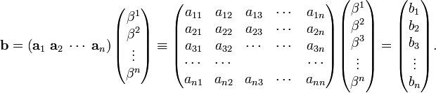
Finally one gets the following expression for the contravariant components of vectors (summation convention!),

$\mathbf{b} = \beta^k \; \mathbf{a}_k \quad \Longrightarrow \quad \beta^k =\langle \mathbf{a}^k \mid \mathbf{b} \rangle \in \mathbb{R},\qquad k=1,2,\ldots, n.$

One recognizes this as Cramer's rule for the solution of {β^k, k=1,2,...,n} from the simultaneous linear equations

$\mathbf{b}= \left(\mathbf{a}_1\;\mathbf{a}_2\;\cdots\; \mathbf{a}_n\right) \begin{pmatrix} \beta^1 \\ \beta^2 \\ \vdots \\ \beta^n\\ \end{pmatrix} \equiv \begin{pmatrix} a_{11} & a_{12} & a_{13} & \cdots & a_{1n} \\ a_{21} & a_{22} & a_{23} & \cdots & a_{2n} \\ a_{31} & a_{32} & \cdots & \cdots & a_{3n} \\ \cdots & \cdots & & & \cdots \\ a_{n1} & a_{n2} & a_{n3} & \cdots & a_{nn} \\ \end{pmatrix} \begin{pmatrix} \beta^1 \\ \beta^2 \\ \beta^3 \\ \vdots \\ \beta^n\\ \end{pmatrix} = \begin{pmatrix} b_1 \\ b_2 \\ b_3\\ \vdots \\ b_n \\ \end{pmatrix}.$

[edit] Notes

↑ A. Einstein, Die Grundlage der allgemeinen Relativitätstheorie [The foundation of the general theory of relativity], Annalen der Physik, Vierte Folge, vol. 49, pp. 769–822 (1916). Downloadable pdf
↑ If the tensor g were singular, its kernel would be non-zero, i.e., there would be a non-zero n-tuple k = (k¹, k², ..., kⁿ) such that
$\mathbf{g} \mathbf{k} = \mathbf{0} \Longrightarrow \ell^i g_{ij} k^j = \ell^i (v_i,v_j) k^j = \left( \ell^i v_i, k^i v_i\right) = (\ell,\; k) = 0,\; \forall \ell \in V_n \Longrightarrow k^1=k^2= \cdots =k^n = 0.$
where the bilinearity of the inner product was used. Contradiction.

[0] A. Einstein, Die Grundlage der allgemeinen Relativitätstheorie [The foundation of the general theory of relativity], Annalen der Physik, Vierte Folge, vol. 49, pp. 769–822 (1916). Downloadable pdf

[1] If the tensor g were singular, its kernel would be non-zero, i.e., there would be a non-zero n-tuple k = (k¹, k², ..., kⁿ) such that
$\mathbf{g} \mathbf{k} = \mathbf{0} \Longrightarrow \ell^i g_{ij} k^j = \ell^i (v_i,v_j) k^j = \left( \ell^i v_i, k^i v_i\right) = (\ell,\; k) = 0,\; \forall \ell \in V_n \Longrightarrow k^1=k^2= \cdots =k^n = 0.$
where the bilinearity of the inner product was used. Contradiction.

[1]

[2]

Dual space (linear algebra)

Contents

[edit] Definition

[edit] The dual of the dual

[edit] Dual transformations

[edit] Matrices

[edit] Basis transformation

[edit] Inner product spaces

[edit] Example

[edit] Application: reciprocal space

[edit] Notes

Personal tools

Namespaces

Variants

Views

Actions

Search

Navigation

Community

Toolbox