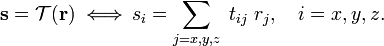
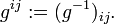
Tensor

Contents |
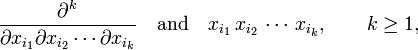
In physics and mathematics, a tensor is an algebraic construct that is defined with respect to an n-dimensional linear space V. Like a vector, a tensor has geometric or physical meaning—it exists independent of choice of basis for V—but yet can be expressed with respect to a basis of V. A k-th rank tensor is represented with respect to a basis of V by an array of nk numbers (the tensor components):

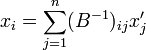
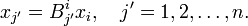
Noteworthy is the special case of a vector, which by definition is a tensor of rank k = 1. A vector in V is represented by an array of numbers {ti | 1 ≤ i ≤ n} (usually written as a column) with respect to a basis of V.
A linear space V is defined with respect to a number field; in physics it is usually the field ℝ of real numbers or the field ℂ of complex numbers. The components of a tensor are in the field of V. A tensor of rank zero is an element of the field of V. In this article only the field ℝ will be considered. Extension to ℂ is usually trivial.
A tensor with respect to V represented by constant numbers is an affine tensor. A tensor with components that are functions of a (position) vector r in V is a tensor field.
[edit] Basis transformation
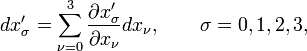
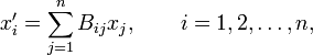
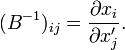
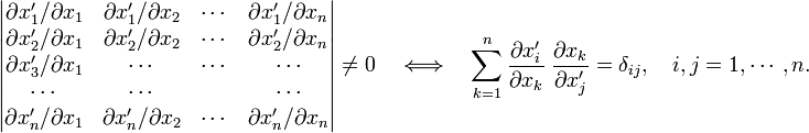
Because a tensor 𝒯 itself is independent of the choice of basis of V, its components ti1i2 ... ik must change under a basis transformation. When another (primed) basis of V is chosen through the basis transformation
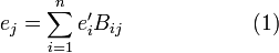
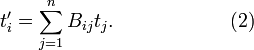
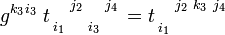
a new array (indicated by a prime) of nk other numbers represents the same k-th rank tensor 𝒯 with respect to the primed basis e′i. A necessary and sufficient condition that an array of nk numbers represents 𝒯 with respect to a basis of a vector space V is: the numbers representing 𝒯 with respect to a primed basis of V must be related by the following equation to the numbers representing 𝒯 with respect to an unprimed basis of V:
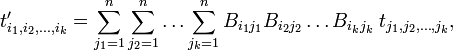
where the matrix B with elements Bij connects the primed and unprimed basis of V as in equation (1). Note the special case: for a tensor of rank k = 1 the equation gives the well-known rule for the transformation of vector components:
[edit] History of tensors
[edit] Early history
The concept of tensor arose in 19th century physics when it was observed that a force (a 3-dimensional vector) applied to a medium (a deformable crystal, a polarizable dielectric, etc.) may give rise to a 3-dimensional response vector that is not parallel to the applied force. One of the first examples was treated by Cauchy (1827) in the case of stress. Some crystalline materials deform in a direction that is not parallel to the applied stress; this is a property of the material; such material is said to be mechanically anisotropic. An electric field applied to an electrically anisotropic material gives a polarization with a direction that is not parallel to the field. The existence of anisotropic materials was considered remarkable, because it required revision of Newton's third law (action is minus reaction): apparently reaction can have a direction that is not along and opposite the action that causes it.[1] In these early days the linear space V mentioned above was always the real 3-dimensional Euclidean space—the concept of higher-dimensional spaces was introduced later in the century. The rank k of the early tensors was almost always equal to two, so that for a long time tensors were represented solely by real 3×3 matrices.
It may be, parenthetically, illuminating to observe that the prototype model of a cause-effect relation is Newton's second law (1687),

This law does not show a tensor behavior at all. The force F causes the acceleration a of a particle; effect and cause are parallel and connected by a scale factor (single real number, tensor of rank zero) m, the mass of the particle; a and F have the same direction.
[edit] Work of Gibbs
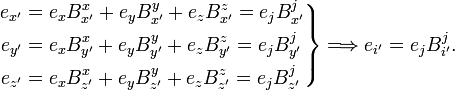
Although Cauchy and others observed tensors early in the 19th century (without giving them a name yet), it took until 1884 before J. Willard Gibbs made some decisive steps.[2] Gibbs considered a linear relation (endomorphism on ℝ3) between the 3-vectors: "cause" r and "effect" s:
and showed that 𝒯—christened by him "dyadic"—can be written in terms of an orthonormal, right-handed, basis i, j, and k of ℝ3,

The "dyadic products" ii, ij, etc. were defined by Gibbs as linear functions of an arbitrary vector r through the inner product defined previously by him. For instance, the following two-term dyadic acting on r gives the response vector as a linear combination of i and k

where j⋅r and k⋅r are inner products (real numbers) between 3-vectors.
In this manner, Gibbs showed that the txx, txy, etc. appear in the prototype tensor relation holding between the components of "cause" r and "effect" s with respect to the same orthonormal basis:
In many physics texts[3] the 3×3 matrix of components tij is called a second rank tensor—more precisely it must be called the representation of the second rank tensor 𝒯 with respect to a basis. It is of some historic interest to point out that it was Gibbs who introduced in 1884 the term "right tensor" for a special form of dyadic, namely a 3×3 tensor described with respect to principal axes. The word "tensor" itself was introduced in the middle 1850s in a different context by Hamilton.[4]
If the coefficients tij do not constitute a identity matrix (or a multiple thereof), the direction of the "cause" r differs from the direction of the "effect" s. When the tij constitute a unit matrix times a scalar, the tensor is called isotropic and the cause and effect vectors are parallel.
[edit] Einstein's definition
Gibbs' second rank tensor 𝒯 exists independent of basis (in applications 𝒯 is usually determined by properties of a material, the geometry of a body, the curvature of a surface, etc., all of which exist prior to choice of basis). As alluded to above, the independence of the tensor 𝒯 on choice of basis implies that its components tij do depend on basis, otherwise the simultaneous transformation of basis and components could not cancel each other. This basis dependence of tensor components gives rise to the definition of tensor that was already given; we will return to it below. It defines a tensor by the behavior of its components under basis transformation. This definition, which was propagated by Einstein,[5] is disliked by mathematicians who prefer a basis-independent definition.
As an additional historical note: in Einstein's general theory of relativity the vector space V is tangent to the curved 4-dimensional space-time continuum. The tangent space V is the four-dimensional Minkowski space that has indefinite metric. Einstein's tensors are tensor fields, i.e., his tensor components are functions of the space-time coordinates (x0, x1, x2, x3). Because he considers fields, Einstein writes equation (2) as
that is, the elements of matrix B effecting the basis transformation are written as differential quotients (first derivatives), which is needed for tensor fields. [For affine tensors the elements in equation (2): Bij = ∂t ′i / ∂tj are constant, independent of the vector components t1, t2,..., tn].
[edit] Mathematical extensions
Without using the term "tensor" (until Einstein made tensors widely known through his work on general relativity theory, only physicists used the term), mathematicians extended Gibbs' concept in two directions:
- Recognizing that 𝒯 belongs to a 9-dimensional tensor product space ℝ3⊗ℝ3, they considered tensor products V⊗W of more general (even infinite dimensional) spaces V and W and more than two factors.
- The transformation properties under a change of basis were generalized to Riemannian manifolds (curved spaces) with local bases (bases of Euclidean tangent spaces). When the local basis is varied over the manifold, a tensor field is obtained.
Especially in the hands of the Italian school of mathematicians, among them Ricci (1853 — 1924) and his student Levi-Civita (1873 — 1941), the theory of what they called Absolute Differential Calculus grew out to a powerful tool in the study of the geometry of curved spaces, usually referred to as differential geometry. Albert Einstein, who referred to the theory by the shorter "tensor calculus",[6][7] [8] found the theory indispensable in his work on general relativity.
[edit] Quantum mechanics
After quantum mechanics was introduced in the middle 1920s, it was soon recognized[9] that a many-particle wave function can be written as a linear combination of tensor products of one-particle wave functions. A few years after the advent of quantum mechanics, John von Neumann showed that quantum mechanical states belong to an infinite dimensional vector space that he christened Hilbert space,[10] so that many-particle states belong to tensor products of (one-particle) Hilbert spaces.
[edit] Physicist's definition
The definition of a tensor by basis transformation will be explained by making the analogy with a vector.
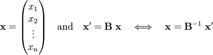
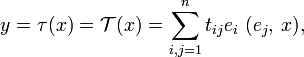
Consider a real n-dimensional vector space V with basis (by definition a maximum linearly independent set of vectors) e1, e2, ..., en. Any vector v in V can be uniquely written as
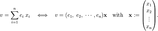
The stack of n real numbers x represents the vector v with respect to the given basis e1, e2, ..., en. What happens to the representation of the given vector v if one chooses a different basis f1, f2, ..., fn? Since bases are linearly independent one can write

so that

where it is used that a basis transformation is invertible. Now,

with I the identity matrix and
Hence, if the stack x represents a vector with respect to a basis, the stack x′ = Bx represents the same vector with respect to a new basis, the one that is transformed by B.
Conversely, suppose a column (stack) x of n real numbers is defined with respect to a given basis of V, say the basis e1, e2, ..., en. Obtain by the same definition a set of numbers x′ with respect to the basis f1, f2, ..., fn that is obtained from {ei} by multiplication with B−1. If it is true that x′ = B x, then both x and x′ represent the same vector. Indeed,

This leads to the (physicist's) definition of a vector:
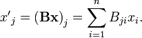
Consider an array of n real numbers x = (x1, x2, ..., xn) defined with respect to a basis of an n-dimensional space V. The array represents a vector (the elements of x are the components of a vector) if and only if the numbers transform asunder a transformation of the basis by B = (Bij).
This definition can be extended to the (physicist's) definition of a tensor:
Consider an array of nk real numbers defined with respect to a basis of an n-dimensional space V. The array represents a kth-rank tensor if and only if the numbers (the tensor components) transform asunder a transformation of the basis by B = (Bij).

Clearly, a vector is a tensor of rank one.
[edit] Mathematician's definition
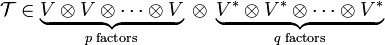
The mathematical definition is simple: a tensor is an element of a certain tensor product space. The difficulty of the definition is shifted to the definition of tensor product space, which preferably is defined without use of basis; different definitions of varying level of mathematical sophistication can be found in the literature. A tensor product of two arbitrary linear spaces V and W is written as V⊗W. Generalization to a product of more than two spaces is by postulating associativity: (U⊗V)⊗W= U⊗(V⊗W) = U⊗V⊗W. (It is irrelevant which pair is multiplied first).
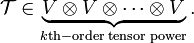
The (purely contravariant) k-th rank tensors (arrays of numbers) considered thus far represent elements in a tensor product space that is constructed from one and the same n-dimensional space V. Stating that an array ti1i2 ... ik represents a k-th rank tensor 𝒯 with respect to V is equivalent to stating that 𝒯 belongs to the tensor power (k-fold product),
When {ei | i=1, ..., n} is a basis for V, the elements

form a basis of nk dimensional tensor power (this holds for any of the equivalent definitions of the tensor product of two linear spaces).
A tensor can be expanded in this basis,
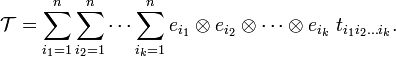
Earlier the component array ti1i2 ... ik was called the representation of 𝒯, the present expansion of 𝒯 in a basis makes the statement explicit.
When the basis of V changes according to equation (1), the basis of tensor power changes as follows (this is a consequence of any of the definitions of tensor product),

It follows immediately that

provided the component array ti1i2 ... ik transforms as a tensor. This shows that, due to the transformation properties of the component array, the tensor 𝒯 does not change under basis transformation.
[edit] Application
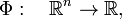
In physical applications (symmetric) tensors appear often in the Taylor-Maclaurin expansion of a scalar-valued function Φ (often an energy) around some point x0 in ℝn (e.g., an equilibrium point),
with

The monomials 1≡xi0 , xi , xjxi , xkxjxi , ... are respectively: a scalar (a zeroth-rank tensor), components of a vector in ℝn (a first-rank tensor), components of a second-rank tensor (represent an element of ℝn⊗ℝn with respect to a basis), components of a third-rank tensor (represent an element of ℝn⊗ℝn⊗ℝn with respect to a basis), etc. The left-hand side is invariant under a transformation of a basis of ℝn and hence the partial derivatives have well-defined transformation properties too (this follows also from the derivatives with respect to xi, xj, etc. having well-defined transformation properties). In other words, the partial derivatives are also tensors, they transform contragrediently to the products xi, xjxi, etc., which means that they "cancel" the transformation of the latter so that the left-hand side is invariant (does not depend on choice of the basis of ℝn).
To make these statements more explicit, consider
where the matrix B, which maps one linearly independent set on another, is non-singular (invertible), i.e., it possesses the inverse B−1. In view of its transformation properties, the quantity

is a component of a tensor of rank k.
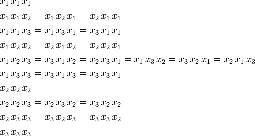
The tensor is symmetric, because, xi and xj being real numbers, it holds that xi xj = xj xi. In general, any permutation of the k subscripts leaves the tensor component invariant. A symmetric tensor has
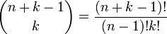
different components. Take as an example n = 3, k = 3 then out of the 3³ = 27 components only 10 are different,
Returning to the basis transformation, it is noted that the matrix element Bij can be written as a partial derivative,

Namely,
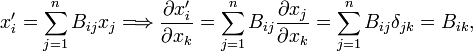
where δjk is the Kronecker delta that appears because the xi are independent. Completely analogously one finds from
that
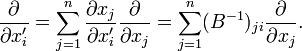
By application of the chain rule for partial differentiation one find for the gradient operators,
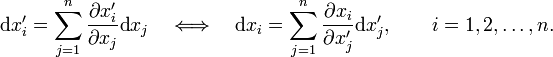
The basis transformation can also be written in terms of differentials:
These differential relations can be seen as the linearizing of the more general, non-linear, basis transformation,

This transformation is invertible—and only then it is a basis transformation—if the Jacobi matrix is invertible, that is, if, and only if, its determinant (the Jacobian) is not equal zero,
Note that the Jacobi matrix is equal to B in the case of a linear basis transformation (for affine tensors).
In summary, for linear basis transformations it holds that,
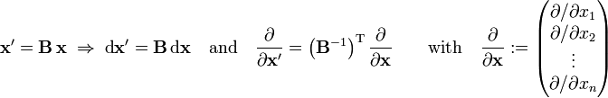
where the superscript T on the matrix B indicates that the transpose of B must be taken. One expresses these equations by stating that x and dx transform contragrediently to ∂/∂x. For non-linear basis transformations the same relations hold provided B is replaced by the Jacobi matrix,

This contragredience shows that individual terms in the Taylor-Maclaurin expansion of a scalar-valued function are invariant under a basis transformation. Indeed,
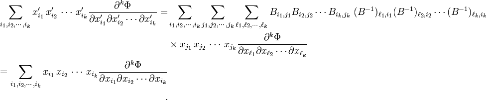
It was used here that
and the remaining summation indices were relabeled to i1, i2, etc. Since for most functions Φ the order of differentiation is immaterial, the kth-order derivatives are also symmetric tensors and it follows that each term in the Taylor-Maclaurin expansion is an invariant product (full contraction of all tensor indices) of two contragredient symmetric tensors. Clearly, Φ does not play a determining role and can be omitted; it follows that
are the components of symmetric k-th rank tensors contragredient to each other.
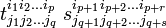
[edit] Mixed affine tensors
Above two kinds of rank-k tensors were discussed: purely contravariant and purely covariant tensors. Now mixed tensors of type  , will be introduced: contravariant of rank p and covariant of rank q. The tensors discussed above were of kind
  and
and  , respectively.
In order to introduce mixed tensors, a change of notation is called for. Two bases of the n-dimensional real vector space V will be introduced. One basis has its elements along unprimed axes (x, y, ... ) and the other basis has its elements along primed axes (x′, y′, ... ). Thus, the bases are:

They are connected through:

where the matrix B of the basis transformation is by definition non-singular, and Einstein's summation convention[5] is introduced. This convention is the following: when an index appears twice in an expression, once as an upper index and once as a lower index, the index is summed over. In the last equation the index j is summed over and i ′ is free. The free indices must appear in the same position (i.e, as lower or upper) in the left- and right-hand side of an equation.
Example of summation convention for a basis transformation in 3-dimensional space,
In this notation the relations (where I is the identity matrix)

are given by

Both indices of the Kronecker δ refer to the same basis, either they both carry a prime, or both are unprimed.
As an example of the notation based on primed subscripts and superscripts and summation convention, the basis transformation
 is inverted.
Multiply both sides by
is inverted.
Multiply both sides by  and sum over i ′,

A vector x ∈ V is written in summation convention as

[edit] Biorthogonal basis
After this intermezzo on notation, it is noted (see dual space) that there are n linear functionals (one-forms) on V, ei, that are biorthogonal (also known as dual) to the basis ej. This means that they are defined as follows

where the bra-ket notation ⟨ . , . ⟩ stands for the action of a linear functional on an element of V (see dual space for more details).
Linear functionals on V constitute a linear space V∗ of dimension n. Elements of this space are bilinear (linear in both arguments) maps of V to ℝ, which means that for instance,

The n elements ej in V∗, biorthogonal to the basis ej of V, form a basis of V∗.
Transform the basis of V by matrix B to a primed basis. Let the basis of the dual space V∗ biorthogonal to the primed basis be indicated by superscripts carrying primes. Let the primed basis of V∗ be obtained by transformation with the matrix D. Hence one has

from which follows that D and B are each others inverse, and hence that the elements of a dual basis transform as components of a vector, compare

These quantities (labeled by upper indices) are said to be contravariant. They transform contragrediently to covariant quantities (labeled by lower indices).
[edit] Definition of mixed tensor
The stage is set for the "physicist's definition" of a mixed tensor of type . A mixed tensor, contravariant of rank p and covariant of rank q, is represented by the following set of np+q real numbers (tensor components):

that are defined with respect to a basis of V and a basis of V∗ biorthogonal to it. When the basis of V is transformed to a primed basis by matrix B and simultaneously the biorthogonal basis of V∗ is transformed by the inverse of B—as discussed above, the following set of numbers

gives the components of the same mixed tensor with respect to the primed basis. This condition is necessary and sufficient that the np+q real numbers are the representation of a tensor.
Note that, in contrast to a basis transformation, which by definition has two indices referring to different bases (a primed and an unprimed index), the tensor components all refer to the same basis, i.e., all components carry a prime, or all are unprimed.
An element of the following tensor product space
can be written as

where the array  is contravariant of rank p and covariant of rank q. By definition 𝒯 itself is invariant and hence the basis is contravariant of rank q and covariant of rank p.
Note: the tensor product is not commutative, in general the space V⊗W is not the same as W⊗V. This implies that elements of, for example,
V⊗V⊗V∗ and V∗⊗V⊗V do not belong to the same space although they are of type  and have the same transformation properties under change of basis of V and V∗.
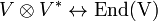
[edit] Mixed tensors as endomorphisms
Often it is loosely stated that a second rank tensor is a matrix. This statement is more accurately rephrased as: a  tensor defined on V is an endomorphism of V. This statement will be proved now.
An endomorphism τ of the real n-dimensional vector space V is a linear map V → V. As is well-known there is a one-to-one correspondence between the algebra End(V) of endomorphisms and the algebra of real n×n matrices M(n,n). The correspondence is defined by a choice of basis ei of V. Upon introduction of summation convention, the correspondence is given by,

First note that an element x∈V can be written as

where ei is an element in a basis dual (biorthogonal) to ei.
Let 𝒯 be in V⊗V∗, that is, 𝒯 is of type . Suppressing for convenience sake the symbol ⊗, we write

The map τ: V → V thus defined is linear. Now

Given a mixed tensor 𝒯, a τ ∈ End(V) is defined. From the tensor character of 𝒯 follows that the definition is independent of choice of basis. Indeed, choose a different (primed basis), then

Conversely, given τ :

Since τ and x are independent of basis, the correspondence τ → 𝒯 is also independent of basis. In summary, there is a one-to-one canonical (basis-independent) map,
and a tensor defined with respect to V can be identified with a linear map on V.
With regard to the historical definition of tensor, 𝒯 can be seen as the map

a linear relation between "cause" x and "effect" y'.
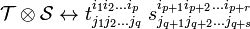
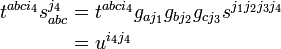
[edit] Multiplication and contraction of tensors
Consider two tensors, 𝒯 of type and 𝒮 of type  , both relative to V. With respect to the same basis of V they have the components

It is clear that the product
transforms a tensor of type  . This tensor is written as
If among the indices of tensor components of type an upper index is put equal to a lower index and (by summation convention) the two indices are summed over, a tensor of type  is obtained. This process is called contraction. Contraction is performed most often among components in a tensor product, say of 𝒯 and 𝒮, and hence we show the procedure for such a product. For convenience sake an example is considered, it will be clear how the result can be generalized to arbitrary tensors.
Thus, consider as an example the tensor product of type  and its transformation property,

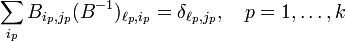
Put, for instance, i′1 = j′3 = k and use
so that
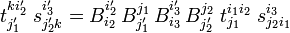
and we see that the tensor contracted over i1

is of type  .
.
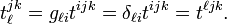
[edit] Raising and lowering of indices
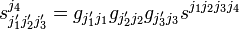
Thus far the space V did not have an inner product. It is now assumed that the real vector space V has a non-degenerate symmetric inner product denoted by ( ⋅, ⋅), which is not necessarily definite. Given a basis {ei } of V, the matrix with elements gij = (ei , ej) is the metric (or fundamental) tensor g. If one transforms g as follows from a primed to an unprimed basis,

one sees that g is a purely covariant  tensor.
It is shown in the article inner product that the metric tensor is invertible. The inverse is a purely contravariant
tensor.
It is shown in the article inner product that the metric tensor is invertible. The inverse is a purely contravariant  tensor, so that it is meaningful to write
It follows by matrix inversion that indeed
![g_{ij} = B^{i'}_{i}B^{j'}_{j} g_{i'j'} \quad\xrightarrow[\scriptstyle\text{invert}]{}\quad
g^{ij} = B_{i'}^{i} B_{j'}^{j} g^{i'j'},](../w/images/math/b/e/4/be41320f03aa6540cde7f10c3ccfde8b.png)
which confirms that the inverse metric tensor is of type . Note that the inverse metric tensor is also symmetric.
Define a new basis εi of V by raising an index, which means that a repeated index in upper and lower position is summed over,

The free index of g determines the type (co- or contravariant) of the result.
The new basis of V is contravariant of type  , that is, it transforms as a vector component,

This is easily verified:
![\epsilon^{i'} = g^{i'j'}\;e_{j'} = [B^{i'}_{i} B^{j'}_{j} g^{ij}]\; [B^{k}_{j'} e_k] = B^{j'}_{j} B^{k}_{j'}\; B^{i'}_{i}g^{ij} \; e_k =
\delta_j^k\; B^{i'}_{i} g^{ij}\; e_k = B^{i'}_{i}\; g^{ik} e_k = B^{i'}_{i}\;\epsilon^i.](../w/images/math/4/5/8/45891581dc909997dda9772809723d5b.png)
By definition the new basis is biorthogonal to the old basis:

The covariant metric tensor can be used to lower an index. Consider, summing again over a co- and contravariant pair of indices,

It is easily verified that xj is covariant,
Clearly, xi and xi represent the same vector x ∈ V with respect to the biorthogonal bases of V.
In order to change the variance of a mixed non-symmetric tensor one can start with a purely contravariant tensor and lower (some of) the indices. In this way one creates vacancies among the upper indices that later can be filled again by raising. For instance,

And raising of the third index:
Clearly, for symmetric tensors the order among the indices is free; one does not have to keep track of vacancies in raising and lowering of indices of symmetric tensors.
Note again that, in contrast to the dual basis ei of the dual space V∗, the present biorthogonal basis εi belongs to the same space as ei and hence the different component arrays with different raised and lowered indices all represent the same tensor. This brings up the question why one would take the effort to raise or lower indices. The answer is: the forming of invariants by contraction. For instance, given two tensors

One can form an invariant from the product of rank less than 8 by lowering indices and contraction (forming partial traces, partial inner products). For example,
and
is a contravariant tensor of type . Clearly, this is a generalization to arbitrary tensors of the inner product between two vectors,

In the article dual space it is shown that when V is equipped with an inner product there is the canonical isomorphism between x ∈ V and x̅ ∈ V∗ defined by

for arbitrary a ∈ V. This isomorphism allows the identification of V with its dual V∗.
[edit] Cartesian tensors
Other than being non-singular, the linear basis transformations, considered so far, were completely arbitrary. If one restricts the attention to transformations from one orthonormal basis to another (in spaces with positive definite inner product), the basis transformations with matrix B are orthogonal,
where the superscript T stands for matrix transposition.
The metric tensor relative to an orthonormal basis is the identity matrix and the raising and lowering of indices becomes an identity operation ("doing nothing"). Because co- and contravariant components become indistinguishable, Einstein's summation convention must be extended to repeated indices, not necessarily in upper and lower position. Thus, for orthogonal matrices it follows that

where summation over repeated index i is implied.
It is verified that orthonormality of a basis is conserved under transformation by an orthogonal matrix,

Tensors of which the components are solely described with respect to orthonormal bases are Cartesian tensors. Their transformation properties are restricted to orthogonal matrices and their co- and contravariant components are equal. Thus, for instance, the Cartesian tensor tijk satisfies
The index ℓ may be seen as contravariant (upper) or covariant (lower).
Earlier it was shown that a mixed tensor 𝒯 of type is essentially an endomorphism τ: V → V,

where ei is an element in a basis of V∗ biorthogonal to ei. With respect to an orthonormal basis, where there is no difference between upper and lower indices, and the basis is biorthogonal to itself, it follows that
which is essentially Gibbs' (1884) expression
In retrospect it may be stated that Gibbs introduced Cartesian tensors in ℝ3.
[edit] References
- ↑ Another breakdown of Newton's third law had been observed also in the early 19th century by Oersted, for the action of an electric current on a compass needle.
- ↑ J. Willard Gibbs, Collected works, vol. 2, part 2, Longmans Green, New York, (1928); p. 17 reprint of: Elements of Vector Analysis, Privately printed, New Haven (1884).Gibbs' definition of tensor online
- ↑ A very early reference is: Woldemar Voigt, Die fundamentalen physikalischen Eigenschaften der Krystalle in elementarer Darstellung, Veit & Co., Leipzig, (1898). Often this work is quoted as the origin of the term tensor.
- ↑ William Rowan Hamilton, On some Extensions of Quaternions
- ↑ 5.0 5.1 A. Einstein, Die Grundlage der allgemeinen Relativitätstheorie [The foundation of the general theory of relativity], Annalen der Physik, Vierte Folge, vol. 49, pp. 769–822 (1916). Downloadable pdf
- ↑ Probably the first to use the term "tensor analysis" was W. Pauli in: Relativitätstheorie in Encyklopädie der Mathematischen Wissenschaften, Vol. 5, Part 2, pp. 539-775, Teubner, Leipzig, (1921).
- ↑ A. Einstein used the term "tensor calculus" in The meaning of relativity, Princeton University Press, (1922); 5th edition, p. 64.
- ↑ It is noteworthy that Levi-Civita added "Calculus of Tensors" to the title of his book when it appeared in English translation: T. Levi-Civita, The Absolute Differential Calculus (Calculus of Tensors), Translated by M. Long, Blackie & Son Ltd. London, (1926). Reprinted by Dover, New York (1977).
- ↑ Hermann Weyl, Gruppentheorie und Quantenmechanik, Hirzel, Leipzig (1928). Second edition (1931) translated by H. P. Robertson as The Theory of Groups and Quantum Mechanics, Methuen, London (1931). Reprinted by Dover, New York (1949)
- ↑ Johann von Neumann, Mathematische Grundlagen der Quantenmechanik [Mathematical Foundations of Quantum Mechanics], Springer, Berlin (1932)