Molecular orbital theory

In chemistry, molecular orbital theory is the theory that deals with the definition and computation of molecular orbitals (MOs). The branch of chemistry that studies MO theory is called quantum chemistry.
The purpose of molecular orbital theory is to obtain approximate solutions of the time-independent Schrödinger equation of molecules—the eigenvalue equation of a molecular Hamiltonian (quantum mechanical energy operator). Solutions of the Schrödinger equation (wave functions) open the door to all kinds of molecular properties of chemical interest.
Molecular orbitals are wave functions describing the quantum mechanical "motion"[1] of one electron in the electrostatic field of all the nuclei of a molecule. In many-electron molecules the electrostatic field due to the positive nuclei is screened (i.e., weakened) by an average electrostatic field due to the negative electrons.
The absolute square |φ|2 (a one-electron density) of an MO φ is usually delocalized, that is, spread out over the whole molecule, hence the adjective "molecular" in the name. This is in contrast to an atomic orbital (AO), which gives rise to a one-electron density localized in the vicinity of a single atom.
In the great majority of MO theories an MO is expanded in a basis χ i of AOs, centered on the different nuclei of the molecule. Let there be Nnuc nuclei in the molecule, let A run over the nuclei and let there be nA AOs on the A-th nucleus, then the MO φ of electron 1 has the following LCAO (linear combination of atomic orbitals) form,
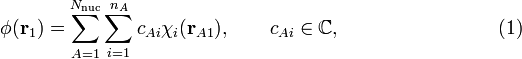
here  is the coordinate vector of electron 1 with respect to a Cartesian coordinate system with nucleus A as origin. Note in this context that nuclei are seen as point charges fixed in space.
Molecular orbital theory deals with the choice of the AOs χ i and the derivation and solution of the equations for the computation of the expansion coefficients cAi. In MO theory the AOs are explicitly known functions (usually algebraic—as opposed to numerical—functions, see this article), and once the expansion coefficients have been determined, the molecular orbitals are known unambiguously and can be used to compute observable molecular properties.
Contents |
[edit] Types of MO theory
A crucial part of MO theory is concerned with the evaluation of molecular integrals (see below). These are 3- and 6-fold integrals over all space that contain as integrands products of AOs, centered on different nuclei, and operators arising from the molecular Hamiltonian. Before 1970, when computers were still in their infancy, the computation of these integrals formed a major hurdle. This is why approximations had to be introduced. Many of these approximations are based on the fact that certain groups of integrals can be seen to represent some empirical (experimentally observable) quantity, usually ionization potentials, electron affinities, or state energy differences. Replacement of groups of integrals by their empirical counterpart (rather than calculation) leads to methods known as semi-empirical MO methods.
When computers and quantum chemical software developed from the 1970s onward, the computation of all necessary molecular integrals became possible. Methods in which all integrals are computed are known as ab initio MO methods. The Latin phrase ab initio stands for from the beginning and implies that no empirical data enter the computation.[2]
An important error in many MO calculations is the neglect of the electronic correlation. By the averaging inherent to Hartree-Fock MO theory, the correlation between the electronic motions is lost. The chance that electron 2 will be near electron 1 is smaller than that it will be far away from electron 1 due to electrostatic repulsion beween the electrons (which falls off with the inverse interelectronic distance). That is, the motion of electron 2 is correlated with the motion of electron 1. Neither ab initio nor semi-empirical MO theory account for this correlation, they treat the electrons as independent particles.
However, there is a one-electron method, density functional theory (DFT) that—at least in principle—accounts of the electronic correlation. Most of the DFT implementations follow Kohn and Sham (KS)[3] who introduced an LCAO expansion into the method. The resulting MOs are often referred to as KS orbitals. So, the KS-DFT method requires a choice of AOs, as do the other MO methods, but also knowledge of the density functional. Since the exact density functional is not known, many different approximations have been proposed, and in that sense DFT is reminiscent of semi-empirical theory with its freedom of choice in empirical parameters.
[edit] Hartree-Fock MO-LCAO theory
[edit] History
In the late 1920s and early 1930s the Briton Hartree[4] and the Russian physicist Fock[5] developed independently an effective one-electron method for the solution of many-electron problems. The method, now known as the Hartree-Fock method (HF), is an iterative method. During the iteration the electron-electron interaction is averaged. Usually (but not always) this is a convergent process. The averaged, converged, electrostatic field due to the electrons is said to be self-consistent. In quantum chemistry the terms Hartree-Fock (HF) and self-consistent-field (SCF) are practically synonyms. Especially Hartree, (often in collaboration with his father William, a retired lecturer of engineering), performed many calculations on atoms. Because of their spherical symmetry atoms are relatively simple: their radial and angular coordinates decouple. The HF equations used then were in operator form—not in matrix form.
Simultaneously, LCAO-MO theory was developed by John Lennard-Jones,[6] Erich Hückel,[7] Friedrich Hund,[8] Robert S. Mulliken,[9] and others. Because of computational difficulties this theory was qualitative or at most semi-quantative, meaning that so many approximations were introduced that the resulting equations were amenable to hand calculations. Symmetry played an important role. By symmetry arguments one can predict when MO coefficients will vanish, or whether some coefficients will be numerically equal.
The HF and LCAO-MO threads were joined in 1951 by the Dutch-American physicist Clemens C.J. Roothaan[10], who wrote the HF equations in a basis of atomic orbitals, thus obtaining matrix equations. It is of course no coincidence that Roothaan performed this work when electronic computers were arriving on the horizon. It is also not a coincidence that Roothaan was at the time working in the University of Chicago Laboratory directed by Robert Mulliken, the great advocate of MO theory.
[edit] Equations
Before sketching their derivation, we present and discuss the Hartree-Fock equations in the form given by Roothaan. Solution of these equations yield the expansion coefficients of Eq. (1). Since in general more than one MO is obtained we enter an extra label to this equation,
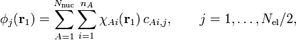
where we assume that each orbital is doubly occupied (once with spin α, once with β) so that the number of occupied MOs is half the number Nel of electrons. The coefficients with fixed j form a column vector in which the rows are labeled by (Ai). Let (Ai) run from 1 to n, that is, denote the total number of AOs by n. We also made a small change in notation by appending the atom label (A) to χ, instead of to the electron coordinate. Both notations can be found in the literature.
The Roothaan equations have the form of a matrix eigenvalue equation, which is not surprising, as the corresponding HF operator equation is also an eigenvalue equation. The matrix to be diagonalized (known as the Fock matrix F ) depends on its eigenvectors. Here enters the same self-consistency procedure as in the original HF problem. First one must guess a set of eigenvectors before the Fock matrix can be constructed. Once the matrix has been constructed, with the guessed eigenvectors as input, it can be diagonalized, i.e., its eigenvectors and eigenvalues can be determined. The computed eigenvectors enter a new iteration cycle in which the Fock matrix is constructed and diagonalized, yielding eigenvectors which (hopefully) are closer to the final result. This procedure is continued until the eigenvectors that enter the Fock matrix are essentially the same as the eigenvectors that emerge from the diagonalization of the Fock matrix. The process is then self-consistent and one has obtained a self-consistent field (SCF).
It must be remarked that the atomic orbitals, localized on different atoms, are non-orthogonal (but linearly independent), while the MOs are constrained to be orthogonal. The non-orthogonality of the basis turns the operator eigenvalue equation into a generalized matrix eigenvalue equation. That is, the matrix equation obtains the form

The Fock matrix F is n × n, the eigenvector matrix C contains Nel/2 columns of length n, the overlap matrix S is n × n and the matrix E is diagonal with the Nel/2 orbital energies on the diagonal. If the AOs were orthonormal, S would be the identity matrix. S contains overlap integrals, which are of the form
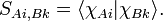
Since  is expressed with respect to a system of axes on atom A,
and
is expressed with respect to a system of axes on atom A,
and  is centered on atom B, this bra-ket is a two-center integral, an integral over
  in which the integrand is expressed with respect to two non-coinciding Cartesian systems of axes.
As is known from linear algebra the matrix S is non-singular (invertible) if and only if the n atomic orbitals are linearly independent. Further S is positive definite in that case (meaning that the Hermitian matrix S has only positive eigenvalues). The matrix F is also Hermitian (usually it is real, in which case the matrix is called symmetric). It is also known from linear algebra that the generalized eigenvalue problem with symmetric F and positive definite S can be solved, i.e., that the columns of C and the corresponding eigenvalues (diagonal elements of E) can be determined. We reiterate: since the AOs χAi are known, after C has been computed the LCAO molecular orbitals φ j have been determined.
[edit] Derivation
With regard to the derivation of the Roothaan equations the following. The derivation applies the variational principle which is based on the fact that the expectation value of the molecular Hamiltonian has a lower bound. An expectation value contains by definition the same wave function in bra and ket. For this function we take a "trial" function containing free parameters that can be varied to minimize the expectation value, and by the boundedness of the Hamiltonian the minimum exists. It is an (unproven) assumption of the variational method that the trial function that minimizes the expectation value gives the best approximation of the exact wave function.
Roothaan took, following Fock, a trial function in the form of a single Slater determinant. Basically this is an antisymmetrized Nel-electron product of spin MOs. In the Slater determinant each spatial MO φ appears twice, once multiplied by the spin function α and once by β. The MOs are expanded as above, and the expansion coefficients serve as variation parameters. When the same Slater determinant is inserted into bra and ket, the expectation value becomes a highly non-linear function of variation parameters. (In fact a Slater determinant is an Nel!-order multinomial in the coefficients and the expectation value is the square of this order). In order to proceed it is necessary to simplify this very complicated expression. At this point one introduces the constraint that the MOs are orthonormal,
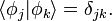
This constraint, for which there is no physical justification, simplifies the derivation considerably. In the 1930s, rules were derived by Slater and Condon & Shortley that allowed the simplification of the expectation value (the so-called Slater-Condon rules). These rules give the reduction of the expectation value to a form that is quartic (fourth power) in the coefficients.
The trick then applied by Roothaan to arrive finally at the matrix eigenvalue equation, was the introduction of the charge- and bond-order matrix (sometimes referred to as density matrix),

which is of dimension n × n. Taking this matrix as given and ignoring the fact that it contains the expansion coefficients, the expectation value becomes quadratic in the coefficients, just as in the linear variation method (also known as Rayleigh-Ritz method). Minimization then yields a matrix eigenvalue equation in the usual manner, with however, a Fock matrix that depends on C through P. In the first iteration P is computed from a guessed matrix C, in following iterations the matrix C is used from the previous iterative step.
[edit] Molecular integrals
The molecular Hamiltonian used in almost all HF calculations does not contain any spin or relativistic terms, but only kinetic energy of the electrons and Coulomb interactions between the electrons and between the nuclei and the electrons. The nuclear Coulomb repulsion is constant because the nuclear geometry is fixed. This also means that the kinetic energy of the nuclei is absent, see Born-Oppenheimer approximation for more details. Thus, three types of integrals appear: kinetic energy, nuclear attraction, and electron repulsion. In the application of the Slater-Condon rules most electron coordinates are integrated over, and what remains are one- and two-electron integrals. Kinetic energy:
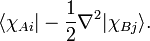
This integral is either a one-center integral (if A = B) or a two-center integral (if A ≠ B).
Nuclear attraction:
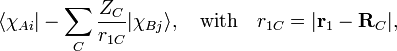
that is, r1C is the distance between electron 1 and nucleus C. Obviously the nuclear attraction integral is at most a three-center integral.
Electron repulsion:

This is a two-electron integral that at most is a four-center integral (A ≠ B ≠ C ≠ D).
Noting that the double index on the AOs runs from 1 to n, we see that there are n4 two-electron integrals. (Actually, if the integrals are real there are some symmetries reducing the number to about n4/8). For fairly small molecules n = 100 is a typical number, leading to 108/8, say 10 million, two-electron integrals. Given the fact that up to four centers are involved and that so many integrals must be calculated, it is not surprising that this part of the MO calculation was a major hurdle for a long time. Initially one tried to use Slater type orbitals for the AOs, but it turned out that three- and four center integrals were almost impossible to calculate with sufficient accuracy. So, now most ab initio MO computer programs use Gaussian type orbitals, which are much easier to integrate.
Initially (in the late 1960s, 1970s, and 1980s when ab initio SCF computer programs were first being written) it was common to precompute all integrals and store them on disk, but in the 1990s it became more efficient to recompute them during the SCF iterations. This is referred to as the direct SCF method. The direct SCF method became more efficient because CPUs developed faster than hard disks and input-output channels. Further it is easier to estimate which integrals can be neglected or computed only approximately when the charge and bond order matrix P (see above) is at hand, so also developments in quantum chemical software made the direct SCF method more attractive. Now, SCF computations with n = 1000 are not uncommon (if the integrals were stored, a terabyte disk would be required).
[edit] Notes and references
- ↑ The quotes are here to remind us that the word motion relates to a stationary, time-independent wave function. In classical mechanics the word motion relates to a time-dependent trajectory. Since quantum mechanics accounts for the (non-zero) kinetic energy of particles the word motion is applicable, but with some care.
- ↑ This name is somewhat pretentious, since the nuclear geometry, (that is, the positions of the nuclei constituting the molecule in space), is often taken from experiment. Further, the choice of AO basis is an art in which experimental data form an important guideline.
- ↑ W. Kohn and L. J. Sham, Self-Consistent Equations Including Exchange and Correlation Effects, Phys. Rev. vol, 140 pp. A1133-A1138 (1965)
- ↑ D. R. Hartree, The Wave Mechanics of an Atom with a Noncoulomb Central Field. Part I. Theory and Methods, Part II. Some Results and Discussions. Proc. Cambridge Phil. Soc., vol. 24, p. 89, 111 (1928)
- ↑ V. A. Fock, Näherungsmethode zur Lösung des quantenmechanischen Mehrkörperproblems. [Approximation method for the solution of the quantum mechanical more-particle problem] Zeitschrift f. Physik, vol. 61, 126 (1930)
- ↑ J. E.Lennard-Jones, The Electronic Structure of some Diatomic Molecules. Trans. Faraday Soc., vol 25, p. 668 (1929)
- ↑ E. Hückel, Quantentheoretische Beiträge zum Problem der aromatischen und ungesättigten Verbindungen: III, [Quantum theoretical contributions to the problem of aromatic and unsaturated compounds] Zeitschrift f. Physik, vol. 76, 628 (1932)
- ↑ F. Hund, Allgemeine Quantenmechanik des Atom- und Molekelbaues [General quantum mechanics of the atom and molecule structure], Handbuch der Physik, 2nd Ed., vol. 24/1, p. 561, Springer, Berlin (1933)
- ↑ R. S. Mulliken, Electronic Structures of Polyatomic Molecules and Valence: Part IV, Electronic States, Quantum Theory of the Double Bond, Phys. Rev. vol. 43, p. 279 (1933)
- ↑ C. C.J. Roothaan, New Developments in Molecular Orbital Theory, Review Modern Physics, vol. 23, p. 69 (1951)
Further reading:
- T. Helgaker, P. Jørgensen, and J. Olsen, Molecular Electronic-Structure Theory, Wiley & Sons, Chichester (2000).
- R. McWeeny, Methods of Molecular Quantum Mechanics, 2nd Ed. Academic Press (1992)
- A. Szabo and N. S. Ostlund Modern Quantum Chemistry: Introduction to Advanced Electronic Structure Theory, Dover, New York (1996)
[edit] External link
The 1929 paper by Lennard Jones