Polarizability

From Knowino

Jump to: navigation, search

In physics, the polarizability of an electric charge-distribution ρ describes the ease by which ρ can be polarized under the influence of an external electric field E.

To explain the concept of polarization of a charge distribution, it is noted that an electric field E is a vector, which by definition "pushes" a positive charge in the direction of the vector and "pulls" a negative electric charge in opposite direction (against the direction of E). Because of this "push-pull" effect the field will distort the charge-distribution ρ, with a build-up of positive charge on that side of ρ to which E is pointing and a build-up of negative charge on the other side of ρ. One calls this distortion the polarization of the charge-distribution. Since it is implicitly assumed that ρ is stable, there are internal forces that keep the charges together. These internal forces resist the polarization and determine the magnitude of the polarizability.

The concept of polarizability is very important in atomic and molecular physics. In atoms and molecules the electronic charge-distribution is stable, as follows from quantum mechanical laws, and an external electric field polarizes the electronic charge cloud. The amount of shifting of charge can be quantitatively expressed in terms of an induced dipole moment.

[edit] Theory

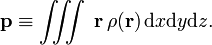
Am electric dipole of a continuous charge-distribution $\rho\,$ is defined as

$\mathbf{p} \equiv \iiint \; \mathbf{r}\, \rho(\mathbf{r}) \, \mathrm{d}x\mathrm{d}y\mathrm{d}z .$

If there is no external field we call the dipole permanent, written as p^perm. A permanent dipole moment may or may not be equal to zero. For highly symmetric charge-distributions (for instance those with an inversion center), the permanent moment is zero.

Under influence of an electric field the charge-distribution will distort and the dipole will change,

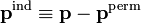
$\mathbf{p}^{\mathrm{ind}} \equiv \mathbf{p}- \mathbf{p}^{\mathrm{perm}}$

where p^ind is the induced dipole, i.e., the change in dipole due to the polarization of the charge-distribution. Assuming a linear dependence in the field, we define the polarizability $\alpha\,$ by the following expression

$\mathbf{p}^{\mathrm{ind}} = \alpha \, \mathbf{E}.$

This relation can be generalized to higher powers in E (in the general case one uses a Taylor series), the polarizabilities arising as factors of E², and E³ are called hyperpolarizabilities and hyper-hyperpolarizabilities, respectively.

The relation above is valid when the vector p is parallel to the vector E, i.e., α is a single real number, a scalar. It can happen that the two vectors (cause and effect) are non-parallel, in that case the defining relation takes the form

$p_i^\mathrm{ind} = \sum_{j=1}^3 \alpha_{ij} \, E_j,$

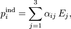
with

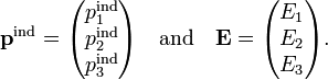
$\mathbf{p}^\mathrm{ind} = \begin{pmatrix}p_1^\mathrm{ind}\\p_2^\mathrm{ind}\\p_3^\mathrm{ind}\end{pmatrix} \quad\hbox{and}\quad \mathbf{E} = \begin{pmatrix}E_1\\E_2\\E_3\end{pmatrix}.$

By writing these two vectors in component form we implicitly assumed the presence of a Cartesian coordinate system. The polarizability α is expressed with respect to the very same coordinate system by a matrix,

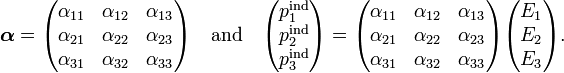
$\boldsymbol{\alpha} = \begin{pmatrix} \alpha_{11} & \alpha_{12} & \alpha_{13} \\ \alpha_{21} & \alpha_{22} & \alpha_{23} \\ \alpha_{31} & \alpha_{32} & \alpha_{33} \\ \end{pmatrix}\quad\hbox{and}\quad \begin{pmatrix}p_1^\mathrm{ind}\\p_2^\mathrm{ind}\\p_3^\mathrm{ind}\end{pmatrix} = \begin{pmatrix} \alpha_{11} & \alpha_{12} & \alpha_{13} \\ \alpha_{21} & \alpha_{22} & \alpha_{23} \\ \alpha_{31} & \alpha_{32} & \alpha_{33} \\ \end{pmatrix} \begin{pmatrix}E_1\\E_2\\E_3\end{pmatrix}.$

We know that choice of another Cartesian basis (coordinate system) changes the column vectors p^ind and E, while the physics of the situation is unchanged, neither the electric field, nor the induced dipole changes, only their representation by column vectors changes. Similarly, upon choice of another basis the polarizibility α is represented by another 3×3 matrix. This means that α is a second rank (because there are two indices) Cartesian tensor, the polarizability tensor of the charge-distribution.

[edit] Units

From the defining equation follows that p has the dimension charge times distance, which in SI units is C m (coulomb times meter). In Gaussian units this is statC cm (statcoulomb times centimeter). An electric field has dimension voltage divided by distance, so that in SI units E has dimension V/m and in Gaussian units statV/cm. Hence the dimension of α is

	SI:	C m² V⁻¹
	Gaussian:	statC cm² statV⁻¹ = cm³,

where we used that in Gaussian units the dimension of V is equal to statC/cm (because of Coulomb's law). In Gaussian units the polarizability has dimension volume, and accordingly polarizability is often considered as a measure for the size of the charge-distribution (usually an atom or a molecule).

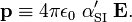
The conversion between the two units is:

$\alpha_{\mathrm{SI}} = \tfrac{10 }{c^2}\;\alpha_{\mathrm{Gaussian}} = 4\pi \epsilon_0\; 10^{-6}\; \alpha_{\mathrm{Gaussian}},$

here c is the speed of light (≈ 3×10⁸ m/s), 4πε₀ = 10⁷/c² (see electric constant) and the suffix on the symbol α indicates the unit in which the polarizability is expressed.

Sometimes one defines the polarizability in SI units by the equation

$\mathbf{p} \equiv 4\pi \epsilon_0\; \alpha'_\mathrm{SI}\; \mathbf{E}.$

This definition has the advantage that α'_SI has dimension volume (m³). Clearly

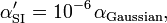
$\alpha'_\mathrm{SI} = 10^{-6} \, \alpha_{\mathrm{Gaussian}},$

where the power of ten is due to converting from m to cm. Sometimes one also encounters the definition

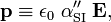
$\mathbf{p} \equiv \epsilon_0\; \alpha''_\mathrm{SI}\; \mathbf{E},$

which gives a polarizability α" with dimension volume and a factor 4π larger than α′.

[edit] Energy

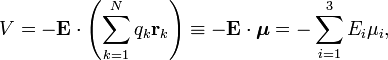
The energy of a dipole in an infinitesimal field is given by

$dU = - \mathbf{p}\cdot \mathrm{d}\mathbf{E} = -(\mathbf{p}^\mathrm{perm} + \mathbf{p}^\mathrm{ind})\cdot\mathrm{d}\mathbf{E},$

where the dot indicates a dot product between the vectors. Integration to finite E gives

$U = - \int_0^{\mathbf{E}} \mathbf{p}\cdot \mathrm{d}\mathbf{E} = -\mathbf{p}^\mathrm{perm} \cdot\mathbf{E} - \frac{1}{2} \alpha \mathbf{E} \cdot\mathbf{E} \equiv U^\mathrm{perm} + U^\mathrm{ind}.$

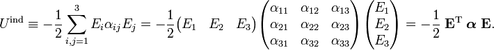
The second term becomes for a non-isotropic polarizibility in three different, but fully equivalent, notations,

$U^\mathrm{ind} \equiv -\frac{1}{2} \sum_{i,j=1}^3 E_i \alpha_{ij} E_j = -\frac{1}{2}\begin{pmatrix} E_1 & E_2 & E_3 \end{pmatrix} \begin{pmatrix} \alpha_{11} & \alpha_{12} & \alpha_{13} \\ \alpha_{21} & \alpha_{22} & \alpha_{23} \\ \alpha_{31} & \alpha_{32} & \alpha_{33} \\ \end{pmatrix} \begin{pmatrix} E_1 \\E_2 \\ E_3 \end{pmatrix} = -\frac{1}{2}\;\mathbf{E}^\mathrm{T} \;\boldsymbol{\alpha}\; \mathbf{E}.$

[edit] Quantum mechanical expression

Classically, electric charge distributions, such as atoms and molecules, were known to exist, but the classical Maxwell theory could not explain their stability. The empirically known polarizability was likewise unexplainable. This changed after the advent of quantum mechanics. By means of the quantum mechanical technique of perturbation theory one can derive an expression for the induction energy U^ind. One introduces a perturbation operator for a system of N particles:

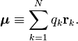
$V = - \mathbf{E}\cdot \left( \sum_{k=1}^N q_k \mathbf{r}_k \right) \equiv -\mathbf{E}\cdot\boldsymbol{\mu} = - \sum_{i=1}^3 E_i \mu_i ,$

where q_k is the charge of the kth particle and r_k its position vector (expressed with respect to some Cartesian coordinate system). Clearly, the dipole operator is defined by

$\boldsymbol{\mu} \equiv \sum_{k=1}^N q_k \mathbf{r}_k .$

In perturbation theory one assumes that the unperturbed (without external field) Schrödinger equations are solved

$H^{(0)} \; \Phi_n = \mathcal{E}_n \Phi_n, \quad n=0,1,\ldots, \quad\hbox{and}\quad \mathcal{E}_0 < \mathcal{E}_1 <\mathcal{E}_2 < \ldots$

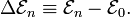
That is, we assume that all states $\Phi_n\,$ and corresponding energies $\mathcal{E}_n$ are known. Further it is assumed that the states constitute an orthonormal basis for the vector space they belong to. The second-order perturbed energy is

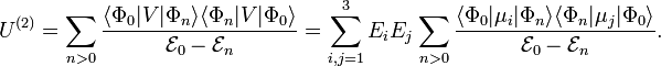
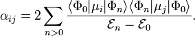
$U^{(2)} = \sum_{n>0} \frac{ \langle \Phi_0 | V | \Phi_n\rangle \langle \Phi_n | V | \Phi_0\rangle}{\mathcal{E}_0 - \mathcal{E}_n} = \sum_{i,j=1}^3 E_i E_j \sum_{n>0} \frac{ \langle \Phi_0 | \mu_i | \Phi_n\rangle \langle \Phi_n | \mu_j | \Phi_0\rangle}{\mathcal{E}_0 - \mathcal{E}_n}.$

Comparing the second-order energy U⁽²⁾ with the induction energy U^ind gives a quantum mechanical expression for the polarizability tensor:

$\alpha_{ij} = 2 \sum_{n>0} \frac{ \langle \Phi_0 | \mu_i | \Phi_n\rangle \langle \Phi_n | \mu_j | \Phi_0\rangle}{\mathcal{E}_n - \mathcal{E}_0} .$

[edit] Frequency-dependent polarizability

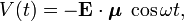
When a charge-distribution is hit by a monochromatic electromagnetic wave with electric component Ecosωt the polarizibility becomes a function of the angular frequency

$\boldsymbol{\alpha}(\omega) \quad\hbox{with}\quad \omega = 2\pi \nu = kc,$

where ν the frequency, k the modulus of the wave vector and c the speed of light. The interaction of the wave with the charge distribution is described by the quantum mechanical operator:

$V(t) = -\mathbf{E}\cdot\boldsymbol{\mu} \; \cos\omega t,$

where the dipole operator μ is defined above. Time-dependent perturbation theory leads to the following expression,

$\alpha_{ij}(\omega) = \sum_{n>0} \left[ \frac{ \langle \Phi_0 | \mu_i | \Phi_n\rangle \langle \Phi_n | \mu_j | \Phi_0\rangle}{\Delta\mathcal{E}_n - \hbar\omega} + \frac{ \langle \Phi_0 | \mu_i | \Phi_n\rangle \langle \Phi_n | \mu_j | \Phi_0\rangle}{\Delta\mathcal{E}_n + \hbar\omega} \right] = \sum_{n>0} \frac{\Delta\mathcal{E}_n \langle \Phi_0 | \mu_i | \Phi_n\rangle \langle \Phi_n | \mu_j | \Phi_0\rangle}{\Delta\mathcal{E}_n^2 - (\hbar\omega)^2},$

where

$\Delta\mathcal{E}_n \equiv \mathcal{E}_n - \mathcal{E}_0.$

The quantity |α(ω)|² is proportional to the cross section for elastic light scattering (Rayleigh scattering), and with a small modification it also gives the cross section for inelastic light scattering (Raman scattering).

The index of refraction n of a charge-distribution is related by the Lorentz-Lorenz relation to its frequency-dependent polarizability α(ω) and hence it follows that n is a function of ω. This leads to the phenomenon of dispersion of light (occurrence of rainbows).

The function α(iω) of imaginary frequency gives rise to one of the components of intermolecular forces, namely dispersion (London) forces.

Polarizability

Contents

[edit] Theory

[edit] Units

[edit] Energy

[edit] Quantum mechanical expression

[edit] Frequency-dependent polarizability

Personal tools

Namespaces

Variants

Views

Actions

Search

Navigation

Community

Toolbox