Virial theorem

From Knowino

Jump to: navigation, search

In mechanics, a virial of a stable system of n particles is a quantity proposed by Rudolf Clausius in 1870.^[1] The virial (from the Latin vis, force) is defined by

$-\tfrac{1}{2} \sum_{i=1}^n \mathbf{r}_i \cdot \mathbf{F}_i ,$

where F_i is the total force acting on the i th particle and r_i is the position of the i th particle; the dot stands for an inner product between the two 3-vectors. Indicate long-time averages by angular brackets. The importance of the virial arises from the virial theorem, which connects the long-time average of the virial to the long-time average ⟨ T ⟩ of the total kinetic energy T of the n-particle system,^[2]

$\langle T \rangle = -\tfrac{1}{2} \sum_{i=1}^n \langle \mathbf{r}_i \cdot \mathbf{F}_i\rangle .$

[edit] Proof of the virial theorem

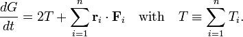
Consider the quantity G defined by

$G \equiv \sum_{i=1}^n \mathbf{r}_i \cdot \mathbf{p}_i\quad \hbox{with}\quad \mathbf{p}_i = m_i \frac{d\mathbf{r}_i}{dt}.$

The vector p_i is the momentum of particle i. Differentiate G with respect to time:

$\frac{dG}{dt} = \sum_{i=1}^n\left[\frac{d\mathbf{r}_i}{dt} \cdot\mathbf{p}_i + \mathbf{r}_i \cdot \frac{d\mathbf{p}_i}{dt} \right]$

Use Newtons's second law and the definition of kinetic energy:

$\mathbf{F}_i = \frac{d\mathbf{p}_i}{dt}\quad \hbox{and}\quad 2 T_i = \frac{d\mathbf{r}_i}{dt}\cdot \mathbf{p}_i$

and it follows that

$\frac{dG}{dt} = 2 T + \sum_{i=1}^n \mathbf{r}_i\cdot\mathbf{F}_i \quad\hbox{with}\quad T \equiv \sum_{i=1}^n T_i.$

Averaging over time gives:

$\left\langle \frac{dG}{dt} \right\rangle \equiv \frac{1}{T} \int_0^T \frac{dG}{dt} dt = \frac{1}{T}\left[ G(T) -G(0) \right].$

If the system is stable, G(t) at time t = 0 and at time t = T is finite. Hence, if T goes to infinity, the quantity on the right hand side, being divided by infinite T, goes to zero. Alternatively, if the system is periodic with period T, G(T) = G(0) and the right hand side will also vanish. Whatever the cause, we assume that the time average of the time derivative of G is zero, and hence

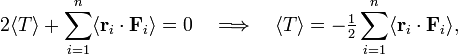
$2 \langle T \rangle + \sum_{i=1}^n \langle \mathbf{r}_i\cdot \mathbf{F}_i \rangle = 0 \quad\Longrightarrow\quad \langle T \rangle = -\tfrac{1}{2} \sum_{i=1}^n \langle \mathbf{r}_i \cdot \mathbf{F}_i\rangle,$

which concludes the proof of the virial theorem: the long-time average of the kinetic energy is equal to the long-time average of the virial.

[edit] Application

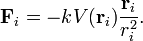
An interesting application arises when the potential V is of the form

$V = \sum_{i=1}^n V(\mathbf{r}_i)\quad \hbox{with}\quad V(\mathbf{r}_i) = a_i r_i ^k\quad\hbox{and}\quad r_i = (x_i^2+y_i^2+z_i^2)^{1/2},$

where a_i is some constant (independent of space and time).

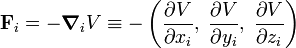
An example of such potential is given by Hooke's law with k = 2 and Coulomb's law with k = −1. The force derived from a potential is

$\mathbf{F}_i = -\boldsymbol{\nabla}_i V \equiv -\left( \frac{ \partial V}{\partial x_i},\; \frac{ \partial V}{\partial y_i},\; \frac{ \partial V}{\partial z_i}\right)$

Consider

$\frac{ \partial V}{\partial x_i} = a_i \frac{ \partial (r_i)^k}{\partial x_i} = a_i k (r_i)^{k-1} \frac{ \partial r_i}{\partial x_i}= a_i k (r_i)^{k-1} \frac{x_i}{r_i} = k \frac{x_i}{r_i^2} V(\mathbf{r}_i).$

Hence

$\mathbf{F}_i = - k V(\mathbf{r}_i) \frac{\mathbf{r}_i}{r_i^2}.$

Then applying this for i = 1, … n,

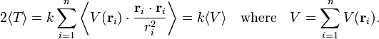
$2\langle T \rangle = k \sum_{i=1}^n \left \langle V(\mathbf{r}_i) \cdot \frac{\mathbf{r}_i\cdot \mathbf{r}_i}{r_i^2}\right\rangle = k\langle V\rangle \quad\hbox{where}\quad V = \sum_{i=1}^n V(\mathbf{r}_i).$

For instance, for a system of charged particles interacting through a Coulomb interaction:

$2\langle T \rangle = - \langle V \rangle.$

For "Hooke particles" (particles in a parabolic potential) it follows that

$\langle T \rangle = \langle V \rangle.$

[edit] Quantum mechanics

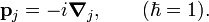
The virial theorem holds also in quantum mechanics. Quantum mechanically the angular brackets do not indicate a time-average, but an expectation value with respect to an exact stationary eigenstate of the Hamiltonian of the system. First the theorem will be proved and then it is applied to the special case of a potential that has a r^k-like dependence. Everywhere Planck's constant ℏ is taken to be one.

Let us consider a n-particle Hamiltonian of the form

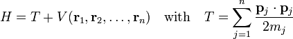
$H = T + V(\mathbf{r}_1, \mathbf{r}_2, \ldots, \mathbf{r}_n)\quad\hbox{with}\quad T = \sum_{j=1}^n \frac{\mathbf{p}_j\cdot\mathbf{p}_j}{2m_j}$

where m_j is the mass of the j-th particle. The momentum operator is

$\mathbf{p}_j = -i \boldsymbol{\nabla}_j, \qquad (\hbar =1).$

Using the self-adjointness of H and the definition of a commutator one has for an arbitrary operator G,

$0 = \langle \Psi | [G, H] | \Psi \rangle\quad\hbox{with}\quad H| \Psi \rangle = E | \Psi \rangle.$

In order to obtain the virial theorem, we consider

$G = \sum_{k=1}^n \mathbf{r}_k \cdot \mathbf{p}_k.$

Use

$[\mathbf{r}_k \cdot \mathbf{p}_k, H] = [\mathbf{r}_k, T] \cdot\mathbf{p}_k + \mathbf{r}_k \cdot[\mathbf{p}_k,V]$

Define

$\mathbf{F}_k \equiv -i [\mathbf{p}_k,V] = - [\boldsymbol{\nabla}_k, V].$

Use

$[r_{k\alpha}, p_{j\beta}^2] = \delta_{kj}\delta_{\alpha \beta} 2 i p_{k \alpha}, \quad \alpha,\beta=x,y,z;\quad k,j=1,,2,\ldots,n,$

and we find

$[G, H] = i\big( 2T + \sum_{j=1}^n \mathbf{r}_j \cdot\mathbf{F}_j \big)$

The quantum mechanical virial theorem follows

$\langle T\rangle = -\tfrac{1}{2} \sum_{j=1}^n \langle \mathbf{r}_j \cdot\mathbf{F}_j \rangle$

where ⟨ … ⟩ stands for an expectation value with respect to the exact eigenfunction Ψ of H.

If V is of the form

$V = \sum_{j=1}^n a_j (r_j)^k,$

it follows that

$\mathbf{F}_j = - [\boldsymbol{\nabla}_j, V] = - a_j\, k \mathbf{r}_j\, (r_j)^{k-2}.$

From this:

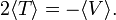
$2\langle T\rangle = k \sum_{j=1}^n a_j \langle (\mathbf{r}_j\cdot\mathbf{r}_j)\, (r_j)^{k-2}\rangle = k \langle V \rangle$

For instance, for a stable atom (consisting of charged particles with Coulomb interaction): k = −1, and hence 2⟨T ⟩ = −⟨V ⟩.

[edit] Reference

↑ R. Clausius, On a Mechanical Theorem applicable to Heat, The London, Edinburgh, and Dublin Philosophical Magazine and Journal of Science, vol. 40, 4th series, pp. 122 – 127 (1870). Google books. Note that Clausius still uses the term vis viva for kinetic energy, but does include the factor ½ in its definition, following Coriolis.
↑ Clausius states this result as: the mean vis viva of the system is equal to its virial.

[0] R. Clausius, On a Mechanical Theorem applicable to Heat, The London, Edinburgh, and Dublin Philosophical Magazine and Journal of Science, vol. 40, 4th series, pp. 122 – 127 (1870). Google books. Note that Clausius still uses the term vis viva for kinetic energy, but does include the factor ½ in its definition, following Coriolis.

[1] Clausius states this result as: the mean vis viva of the system is equal to its virial.

[1]

[2]

Virial theorem

Contents

[edit] Proof of the virial theorem

[edit] Application

[edit] Quantum mechanics

[edit] Reference

Personal tools

Namespaces

Variants

Views

Actions

Search

Navigation

Community

Toolbox