Levi-Civita symbol

In mathematics, a Levi-Civita symbol (or permutation symbol) is a quantity marked by n integer labels. The symbol itself can take on three values: 0, 1, and −1 depending on its labels. The symbol is called after the Italian mathematician Tullio Levi-Civita (1873–1941), who introduced it and made heavy use of it in his work on tensor calculus (Absolute Differential Calculus).
Contents |
[edit] Definition
The Levi-Civita symbol is written as

The symbol designates zero if two or more indices (labels) are equal. If all indices are different, the set of indices forms a permutation of {1, 2, ..., n}. A permutation π has parity (signature): (−1)π = ±1; the Levi-Civita symbol is equal to (−1)π if all indices are different. Hence

else

Example
Take n = 3, then there are 33 = 27 label combinations; of these only 3! = 6 give a non-vanishing result. Thus, for instance,

while

[edit] Application
An important application of the Levi-Civita symbol is in the concise expression of a determinant of a square matrix. Write the matrix A as follows:
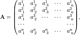
then the determinant of A can be written as:

where Einstein's summation convention is used: a summation over a repeated upper and lower index is implied. (That is, there is an n-fold summation over i1, i2, ..., in).
[edit] Properties
Very useful properties in the case n = 3 are the following,
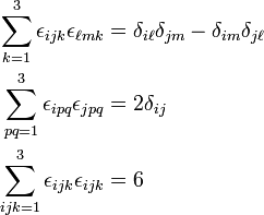
Note that the sum in the first expression contains one non-zero term only: if i ≠ j there is one value left for k for which εijk ≠ 0. The same holds for the second factor in the first expression. The sum over k is a convenient way of picking the value of k that gives a non-vanishing result. The double sum in the second expression is over two non-zero terms: εipqεjpq and εiqpεjqp. The triple sum in the third expression is over 3!=6 non-zero terms.
[edit] Proof
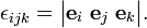
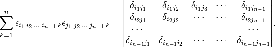
The proof of the properties is easiest by observing that εijk can be written as a determinant. This also opens the way to a generalization for general n > 3.
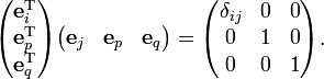
Write
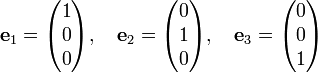
Obviously, the unit columns are orthonormal,
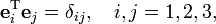
where δij is the Kronecker delta.
Consider determinants consisting of three columns selected out of the three unit columns. Then by the properties of determinants:

Further,

Hence
Introduce 3×3 matrices A and B as short-hand notations:

Use
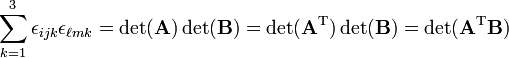
and
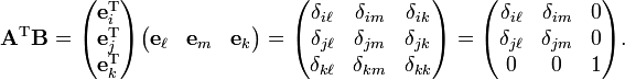
The zeros in the third column appear because i ≠ k and j ≠ k. (If this were not the case εijk = 0). A similar reason explains the zeros in the third row. Hence,
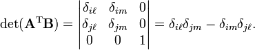
A generalization of the property to arbitrary n is clear now:
The second property of the Levi-Civita symbol follows from
The determinant of the last matrix is equal to δij. The same holds for p and q interchanged. In the case of general n the sum is over (n−1)! permutations [note that (3-1)!=2]. The final property contains a summation over six (3!) non-zero terms; each term is the determinant of the identity matrix, which is unity.
[edit] Is the Levi-Civita symbol a tensor?
In the physicist's conception, a tensor is characterized by its behavior under transformations between bases of a certain underlying linear space. If the most general basis transformations are considered, the answer is no, the Levi-Civita symbol is not a tensor. If, however, the underlying space is proper Euclidean and only orthonormal bases are considered, then the answer is yes, the Levi-Civita symbol is a tensor.
In order to clarify the answer, it is necessary to consider how the Levi-Civita symbol behaves under basis transformations.
[edit] Transformation properties
Consider an n-dimensional space V with non-degenerate inner product. Let two bases of this space be connected by the non-singular basis transformation B,

where by summation convention a sum over ik is implied. The primes indicate a set of axes and may not be used for anything else. An arbitrary vector a∈V has the following components with respect to the two bases:
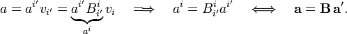
Consider a set of n linearly independent vectors with columns ak and a′k with respect to the unprimed and primed basis, respectively,

Take determinants,

Use
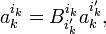
for k = 1, 2, ..., n, successively. Then

Since the component vectors a′k are linearly independent, the coefficients of the powers of ai ′i may be equated and the following transformation rule for the Levi-Civita symbol results,

Except for the factor det(B), the symbol transforms as a covariant tensor under basis transformation. When only transformations with det(B) = 1 are considered, the symbol is a tensor. If det(B) can be ±1 the symbol is a pseudotensor.
It is convenient to relate det(B) to the metric tensor g. An element of g′ is given by (where parentheses indicate an inner product),

Take determinants,
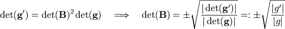
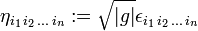
Insert the positive value of det(B) into the transformation property of the Levi-Civita symbol,

then clearly the quantity ηi1 i2...in defined by
transforms as a covariant tensor. If det(B) is negative, ηi1 i2...in acquires an extra minus sign upon transformation, so that ηi1 i2...in is a pseudotensor. For the record,
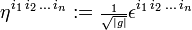
is a contravariant pseudotensor.
Let the inner product on V now be positive definite (and the space V be proper Euclidean) and consider only orthonormal bases. The matrix B transforming an orthonormal basis to another orthonormal basis, has the property BTB = I (the identity matrix). Hence BT = B−1, i.e., B is an orthogonal matrix. From det(BT) = det(B) = det(B−1) = det(B)−1 follows that an orthogonal matrix has determinant ±1. Provided only orthogonal basis transformations are considered, the Levi-Civita symbol is either a tensor [if transformation are restricted to det(B)=1] or a pseudotensor [det(B)=−1 is also allowed]. The orthogonal transformations form a group, the orthogonal group in n dimensions, designated by O(n); its special [det(B)=1] subgroup is SO(n). The Levi-Civita symbol is an SO(n)-tensor (sometimes referred to as Cartesian tensor) and an O(n)-pseudotensor.