Symbolic Logic:Learning:Inductive Inference

[edit] Purpose of web page
This page is an attempt to put together a simple description of Inductive Inference.
Inductive inference is the theory of learning, in a general form. The purpose is to create a theoretical description of Inductive Inference.
I wanted to be able to assign probabilities to real world events. The only basis for such probabilities is the past history of data. So the problem is, given a history of data predict future data.
[edit] Summary
Bayes law is a well established probability law that allows the inference of future events from past history. Unfortunately Bayes law requires the existence of prior probability distributions.
Information Theory gives us some kind of an answer and explanation to this difficulty. A direct link is established between the length of optimally encoded data and their probabilities. This allows us to relate prior probabilities to the size of the model and the conditional probability to the size of the message. The two are needed to transmit the full message, or to give a estimate of the whole probability.
The probabilities of models (represented as optimally encoded data) may be interpreted as priors to Bayes' law. This gives an Inductive Inference framework. The inclusion of the probabilities of the models is seems as key to avoiding over-fitting.
[edit] Inductive Inference
A general theory is described below, by which probabilities may be assign to events based on the data history available.
The theory does not make assumptions about the nature of the world, the fairness of coins, or other things. Instead based solely on the data the theory should be able to assign probabilities.
The problem may be simplified as follows;
Given the first N bits of a sequence assign probabilities to bits that come after it.
In general the input data may not be a sequence of bits. It may be a sequence of real numbers, or an array of data representing images. But all such data may be reduced to a sequence of bits, so for this discussion the simplification of the problem is adequate.
The theory assigns probabilities to models of the data. Each model is a function that maps model parameters to a data sequence. In addition a model may take a series of code bits as input to the model.
The theory is applicable to machine intelligence at a theoretical level. In practice there are computability problems.
[edit] Probabilities based on Message Length
In general the shorter the description of a theory that describes some data the more probable the theory. This principle is called Occam's razor. This is described in,
All these theories give ways of measuring how good a model is. The shortest complete representation of the original data is the most likely to be correct. A complete representation is a data we could send to somebody else to reconstruct the original data. This data is often expressed as data describing a model plus data describing the actual data using the modal.
There is a kind of infinite regress here. The model must be described in a language known to the receiver. In fact inductive inference has problems due to this infinite regress.
[edit] Probability of a mesage
When we send message we need to know where the end of the message is. This end point must be marked within the message. This means that no message may start with another message. If a message started with the complete data from another of a message we would conclude that it had ended with that message. This means the messages must be Prefix Codes.
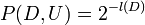
For a prefix code X optimally encoded according to its underlying probability distribution, it's probability P(X) can be determined from it's length l(X) using,
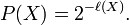
or,
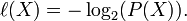
Where l(X) is the length of X. An optical encoded message appears as random data. l(X) bits has 2l(X) states. Given optimal encoding each state has the same probability. So,
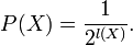
If every leaf of the prefix tree is used the sum of the probabilities of the prefix codes is 1. See Huffman Encoding for the probabilitie description of the prefix tree.
[edit] Models + Codes
In compressing data we want an encoding function that chooses a representation for a message based on its probability.
raw data D --> encoding function e --> compressed data code C
The encoding function e must know the probability of the message D in order to compress it to its optimal encoding. The probability function is called the model M.
The encoding function e must give optimal compression of the data D, given probabilities described by the model M. See Arithmetic Encoding. How the encoding function works is unimportant for the calculating probabilities.
The model function is needed to uncompress the code. So the model function is part of the code. It must be represented with a series of bits of length l(M). The model must also be encoded optimally based on an a-priori probability distribution available.
The model M and the code C are needed to reconstruct the original message D. I will write M + C to mean the model M with the the code C appended.

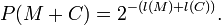

The length l(M + C) is what Occam's Razor tells us to minimise.
[edit] Probabilities of Models
The probability of a model is related to the length of its optimal encoding. If there was a language for describing models that had evolved to give an optimal encoding of models we could use it to give prior probabilities for models.
What we have instead is mathematics, which has evolved through unknown processes. We can guess that mathematics has evolved in general terms to give an efficient encoding of real world data. So with some sensible compression applied to it mathematics is an approximation to an optimal encoding strategy that gives real world prior probabilities.
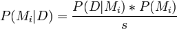
[edit] Bayes Theorem
Bayes' Theorem can be extended to cover a partition of events. This is not difficult once conditional probabilities are understood. This is explained in Bayes' theorem alternate form. See also *Bayes' theorem.
Given a set of alternatives,
- Ai are mutually exclusive sets of events (a Partition) where i is in the set K.
- B is a set of events.
- P(B | Ai) is the probability of B given Ai.
- P(Ai | B) is the probability of Ai given B.
then,
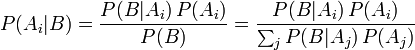 .
.
[edit] Probability Theory Terminology
An Experiment has a set of Outcomes. These outcomes are classified into sets called Events.
[edit] The Universe Generator
Assume that the data sequence was generated from some model. A model assigns a probability to each data sequence.
- A data sequence, tagged with the model it is generated from is an outcome. The same data sequence from two different models are defined to be different outcomes.
- A model is an event.
- A data sequence prefix D is an event.
We can think of the experiment as a two step process.
- 1 - A model P(Mi) is created with probability,
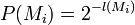
- 2 - A data sequence is generated from the model.
This outcome belongs to the event D of outcomes with this prefix. The model has a probability of generating this data set,
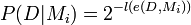
where e(D,Mi) represents the encoding of D with the model Mi.
Bayes' Theorem may be applied to this experiment. Each outcome is tagged with the model it is created from, so the models Mi are a Partition of the set of all outcomes.
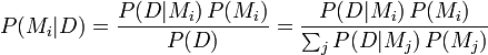 .
.
This gives the probability that the outcome was generated by the model given a data prefix D.
[edit] Predictive Models
Some models will compress the data,
- P(D,Mi) * P(Mi) > P(D)
- l(e(D,Mi)) + l(Mi) < l(D)
These are the models that provide information about the behaviour of D, by compressing the data. They are predictive models.
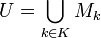
Other models dont compress the data. These are unpredictive models. Rather than deal with each unpredictive model separately we want to group them together and handle them all as the set U of models that dont compress the data. Two sets of indexes J and K are created for the good and bad models,

is the set of indexes of models that compress the data.

is the set of indexes of models that dont compress the data.
The term model has multiple meanings. A model is a probabiliy function for data generated from the model. But it also identifies the set of outcomes generated from the model (the model event). We define U as the union of the model events for which no data compression happens on the data history D.
Then we need to know,
Bayes law with all the models that dont compress the data merged together becomes,
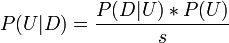
where
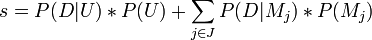
summarising the probabilities,
| P(Mi | D) | is the probability the model i is correct. |
| P(U | D) | is the probability that the data is incompressible. |
| P(D | Mi) | 
|
| P(Mi) | 
|
| P(D | U) | 
|
| P(U) | 
|
| P(D | Mj) * P(Mj) | 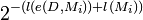
|
[edit] Predicting the Future
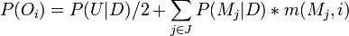
Based on the probabilities of the models found by the methods above we can find a probability distribution for future events.
Each model j predicts a probability  for the i th bit of future data. The probability of a bit i being set in the outcome O is,
[edit] Examples
This section gives examples.
[edit] Two Theories
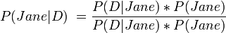
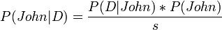
Suppose there is a murder mystery and we know that only Jane had access to murder the victim. Then we feel that we have good evidence that Jane did the deed. But if later on we find that John also had access then the probability that Jane did it suddenly halves.
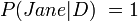
If we only have "Jane did it" as a theory,

And so
But if "John did it" and "Jane did it" are equally complex,

And so

[edit] Regression
Inductive Regression is a sub field of Inductive Inverence which deals with continuous variables. It is an example of Inductive Inference.
[edit] The Frequentist View
We have attempted to describe an experiment, and apply well accepted probability laws to it. It is unusual that there is only one trial, but I dont see this as invalidating the approach. I dont see any basis for saying that we have made a different or Bayesian interpretation of probability. We have simply applied well established laws of probability.
[edit] Conclusion
The above methods for calculating the probabilities of future events based on past history may be considered to be an inductive framework.
There is a level of discomfort in the framework, even though each step seems logical. Firstly the calculation of inferred probabilities seems impractically difficult. Secondly the language used to describe the models may not give an optimal encoding, and only gives an approximation for the prior probabilities of models.
It seems that the use of Inductive Inference requires us to lower our expectation of what probability means from being an absolute measure, to a measure relative to a particular set of prior assumptions.
In practice I would say an inductive probability is a function of,
- The event
- The history
- The language used to encode the models.
[edit] Links
[edit] References
- Inductive inference
- Occam's razor
- Kolmogorov complexity
- Minimum message length
- Minimum description length
- Information Theory
- Claude Shannon
- Kraft's inequality
- Bayes' theorem alternate form