Spherical well

In quantum mechanics the spherical well problem is to find the energy eigenstates and values of a single particle of mass m constrained within a potential that is zero inside a sphere centred on the origin, and infinite outside that region. A classical analogy would be to imagine a grain of sand inside a tennis ball; the grain is free to move anywhere inside but cannot pass through the hard wall of the ball. Applications in quantum mechanics include nucleons in atomic nuclei, or alpha radioactivity where the barrier is not infinite and the particle tunnels through it.
You could argue that the problem can be made more general by allowing the sphere to be centred at an arbitrary location instead of the origin, and by setting the potential inside the sphere to some value V0 instead of 0. However neither of these changes affects the physics of the problem, since we are free to perform a coordinate transformation to put the origin back at the centre of the sphere, and we are free to choose the zero reference point for our energy scale anywhere. This is because only energy differences are actually important, not the absolute values that we apply to them. Since outside the sphere the potential is infinite, the difference between outside and inside is also infinite no matter what energy we choose to label the inside with.
We will continue then with the original problem, of a spherical region of zero potential centred at the origin, with the potential infinite everywhere else.
[edit] Mathematical description
The potential in this problem is best described mathematically in spherical coordinates, as
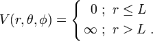
This describes the region in which the particle can exist as a sphere of radius L centred at the origin; outside the ball the potential is infinite, as discussed above. Note that this means the potential is independent of θ and  .
.
The 3D time-independent Schrödinger equation for this system is
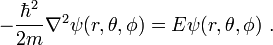
Due to the spherical symmetry of the Hamiltonian the wavefunction can be written as

and then the technique of separation of variables results in two differential equations to be solved, one for R and one for Y. It turns out that the solutions for R are given by the spherical Bessel functions, Jn(r), and the solutions for Y are the spherical harmonics,  .
This gives us three quantum numbers, n,l,m, as opposed to the single quantum number n obtained in the one-dimensional case above. The solution to the spherical well is then
.
This gives us three quantum numbers, n,l,m, as opposed to the single quantum number n obtained in the one-dimensional case above. The solution to the spherical well is then

Should add energy eigenvalues too
[edit] The derivation
The Laplacian in spherical coordinates is given by

We can solve this problem using separation of variables. Since the potential depends on r but not θ or we postulate that the wavefunction ψ can be separated into a product of two functions, one depending on r and the other depending on θ and ,
which turns the Laplacian of the wavefunction into
![\begin{align}\nabla^2\psi &=
\frac{Y}{r^2}\frac{\partial}{\partial r}\left(r^2\frac{\partial R}{\partial r}\right)
+\frac{R}{r^2\sin\theta}\frac{\partial}{\partial\theta}\left(\sin\theta\frac{\partial Y}{\partial\theta}\right)
+\frac{R}{r^2\sin^2\theta}\frac{\partial^2 Y}{\partial\phi^2} \\
&=
\left[
\frac{1}{Rr^2}\frac{\partial}{\partial r}\left(r^2\frac{\partial R}{\partial r}\right)
+\frac{1}{Y r^2\sin\theta}\frac{\partial}{\partial\theta}\left(\sin\theta\frac{\partial Y}{\partial\theta}\right)
+\frac{1}{Y r^2\sin^2\theta}\frac{\partial^2Y}{\partial\phi^2}
\right]\psi\ .
\end{align}](../w/images/math/5/5/1/55187c3f03d5da493bf8d59f7cd87c92.png)
We can now cancel ψ from both sides of Schrödinger equation above, giving us

The variables are finally separated once we multiply through by r2 and rearrange the equation to give
![\frac{1}{R}\frac{\partial}{\partial r}\left(r^2\frac{\partial R}{\partial r}\right)
+\frac{2mEr^2}{\hbar^2}
=
-\frac{1}{Y}\left[
\frac{1}{\sin\theta}\frac{\partial}{\partial\theta}\left(\sin\theta\frac{\partial Y}{\partial\theta}\right)
+\frac{1}{\sin^2\theta}\frac{\partial^2 Y}{\partial\phi^2}
\right]=\alpha](../w/images/math/e/f/2/ef2f5f543037dc4e2eb944e0c2a826a1.png)
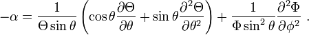
in which the left-hand side only depends on r while the right-hand side depends on θ and instead. This means that when r is varied on the left-hand side the right-hand side will remain constant, and similarly the left-hand side is unaffected by variations of the angular variables on the right-hand side. Therefore both sides must be constant in general, and we have called this constant α. Evaluating the derivative in the first term we find
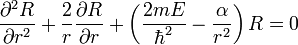
...
Solutions are Bessel functions...
to be continued...
Now we look to the second term. We again want to use separation of variables so let 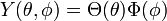 ,
which gives us
,
which gives us
The θ and terms can indeed be separated:
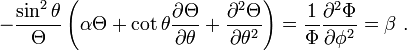
Let's deal with the DE in first,
Now, we know that represents an angular coordinate so we should have that
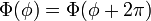 , which yields

or

Since this must hold true for all values of , the bracketed terms must both be zero.
(To see this more explicitly, consider the two specific equations that arise from  and
and  .)
We have shown then that
.)
We have shown then that  must be true,
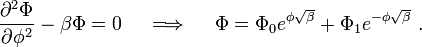
which tells us that
must be true,
which tells us that  , or β = − m2, where m is any integer.
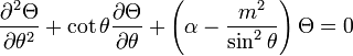
This means that our equation in θ has become
, or β = − m2, where m is any integer.
This means that our equation in θ has become
...
Solutions are Legendre polynomials...
to be continued...
| |
Some content on this page may previously have appeared on Citizendium. |