Rotating wave approximation

From Knowino

This is a pending revision of this page. It may differ from the latest accepted revision, which was accepted on 22 December 2010.

Pending changes are displayed on this page

Jump to: navigation, search

The rotating wave approximation is frequently used in quantum optics, usually to simplify problems involving lasers interacting with atoms. The typical situation involves a coherent (classical) laser light field of frequency $ω L$ and a two-level atom with resonant frequency $ω 0$ . Since little will happen if the laser is not near resonance, the interesting case is when $\omega_L\approx\omega_0$ . In this case, terms with the sum frequency $Σ: = ω L + ω 0$ are discarded under the rotating wave approximation because they oscillate much more quickly than terms with the difference frequency $Δ: = ω L - ω 0,$ which is approximately zero. Note that $Δ$ is by definition the detuning of the laser field with respect to the atomic transition.

The name of the approximation stems from the fact that we switch to the interaction picture where terms oscillating at the frequencies $Σ$ and $Δ$ arise in the Hamiltonian. By transforming to this picture the evolution of the atom due to the corresponding atomic Hamiltonian is absorbed into the system ket, leaving only the evolution due to the interaction of the atom with the light field to consider. Since it is in this picture that the rapidly-oscillating terms mentioned previously can be neglected, and in some sense the interaction picture can be thought of as rotating with the system ket, only that part of the electromagnetic wave that approximately co-rotates is kept; the counter-rotating component is discarded.

[edit] Mathematical formulation

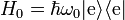
For simplicity consider a two-level atomic system with excited and ground states $|\mathrm{e}\rangle$ and $|\mathrm{g}\rangle$ respectively (using the Dirac bracket notation). Let the energy difference between the states be $\hbar\omega_0$ so that $ω 0$ is the transition frequency of the system. Then the unperturbed Hamiltonian of the atom can be written as

$H_0=\hbar\omega_0|\mathrm{e}\rangle\langle\mathrm{e}|$

Suppose the atom is placed at $z = 0$ in an external (classical) electric field of frequency $ω L$ , given by $\vec{E}(z,t)=\vec{E}_0(z)e^{-i\omega_Lt}+\vec{E}_0^*(z)e^{i\omega_Lt}$ (so that the field contains both positive- and negative-frequency modes in general). Then under the dipole approximation the interaction Hamiltonian can be expressed as

$H_I=-\vec{d}\cdot\vec{E}$

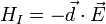
where $\vec{d}$ is the dipole moment operator of the atom. The total Hamiltonian for the atom-light system is therefore $H = H 0 + H I .$ The atom does not have a dipole moment when it is in an energy eigenstate, so 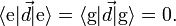$\langle\mathrm{e}|\vec{d}|\mathrm{e}\rangle=\langle\mathrm{g}|\vec{d}|\mathrm{g}\rangle=0.$ This means that defining 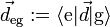$\vec{d}_{\mathrm{eg}}:=\langle\mathrm{e}|\vec{d}|\mathrm{g}\rangle$ allows the dipole operator to be written as

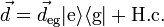
$\vec{d}=\vec{d}_{\mathrm{eg}}|\mathrm{e}\rangle\langle\mathrm{g}|+\mathrm{H.c.}$

(with `H.c.' denoting the Hermitean conjugate). The interaction Hamiltonian can then be shown to be (see the Derivations section below)

$H_I=-\hbar\left(\Omega e^{-i\omega_Lt}+\tilde{\Omega}e^{i\omega_Lt}\right)|\mathrm{e}\rangle\langle\mathrm{g}| -\hbar\left(\tilde{\Omega}^*e^{-i\omega_Lt}+\Omega^*e^{i\omega_Lt}\right)|\mathrm{g}\rangle\langle\mathrm{e}|$

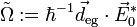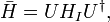
where $Ω$ is the Rabi frequency and $\tilde{\Omega}:=\hbar^{-1}\vec{d}_\mathrm{eg}\cdot\vec{E}_0^*$ is the counter-rotating frequency. To see why the $\tilde{\Omega}$ terms are called `counter-rotating' consider a unitary transformation to the interaction or Dirac picture where the transformed Hamiltonian $\bar{H}$ is given by

$\bar{H}=-\hbar\left(\Omega e^{-i\Delta t}+\tilde{\Omega}e^{i\Sigma t}\right)|\mathrm{e}\rangle\langle\mathrm{g}| -\hbar\left(\tilde{\Omega}^*e^{-i\Sigma t}+\Omega^*e^{i\Delta t}\right)|\mathrm{g}\rangle\langle\mathrm{e}|\ .$

[edit] Making the approximation

This is the point at which the rotating wave approximation is made. The dipole approximation has been assumed, and for this to remain valid the electric field must be near resonance with the atomic transition. This means that $\Delta\ll\Sigma$ and the complex exponentials multiplying $\tilde{\Omega}$ and $\tilde{\Omega}^*$ can be considered to be rapidly oscillating. Hence on any appreciable time scale the oscillations will quickly average to 0. The rotating wave approximation is thus the claim that these terms are negligible and the Hamiltonian can be written in the interaction picture as

$\bar{H}_\mathrm{RWA}=-\hbar\Omega e^{-i\Delta t}|\mathrm{e}\rangle\langle\mathrm{g}| -\hbar\Omega^*e^{i\Delta t}|\mathrm{g}\rangle\langle\mathrm{e}|\ .$

Finally, in the Schrödinger picture the Hamiltonian is given by

$H_\mathrm{RWA}=\hbar\omega_0|\mathrm{e}\rangle\langle\mathrm{e}| -\hbar\Omega e^{-i\omega_Lt}|\mathrm{e}\rangle\langle\mathrm{g}| -\hbar\Omega^*e^{i\omega_Lt}|\mathrm{g}\rangle\langle\mathrm{e}|\ .$

At this point the rotating wave approximation is complete. A common first step beyond this is to remove the remaining time dependence in the Hamiltonian via another unitary transformation.

[edit] Derivations

Given the above definitions the interaction Hamiltonian is

$H_I = -\vec{d}\cdot\vec{E}$

$=-\left(\vec{d}_\mathrm{eg}|\mathrm{e}\rangle\langle\mathrm{g}|+\vec{d}_\mathrm{eg}^*|\mathrm{g}\rangle\langle\mathrm{e}|\right) \cdot\left(\vec{E}_0e^{-i\omega_Lt}+\vec{E}_0^*e^{i\omega_Lt}\right)$

$=-\left(\vec{d}_\mathrm{eg}\cdot\vec{E}_0e^{-i\omega_Lt} +\vec{d}_\mathrm{eg}\cdot\vec{E}_0^*e^{i\omega_Lt}\right)|\mathrm{e}\rangle\langle\mathrm{g}| -\left(\vec{d}_\mathrm{eg}^*\cdot\vec{E}_0e^{-i\omega_Lt} +\vec{d}_\mathrm{eg}^*\cdot\vec{E}_0^*e^{i\omega_Lt}\right)|\mathrm{g}\rangle\langle\mathrm{e}|$

$=-\hbar\left(\Omega e^{-i\omega_Lt}+\tilde{\Omega}e^{i\omega_Lt}\right)|\mathrm{e}\rangle\langle\mathrm{g}| -\hbar\left(\tilde{\Omega}^*e^{-i\omega_Lt}+\Omega^*e^{i\omega_Lt}\right)|\mathrm{g}\rangle\langle\mathrm{e}|\ ,$

as stated. The next stage is to find the Hamiltonian in the interaction picture, $\bar{H}.$ The unitary operator required for the transformation is $U=e^{iH_0t/\hbar},$ and an arbitrary state $|\psi\rangle$ transforms to $|\bar{\psi}\rangle=U|\psi\rangle.$ The Schrödinger equation must still hold in this new picture, so

$\bar{H}|\bar{\psi}\rangle =i\hbar\partial_t|\bar{\psi}\rangle =i\hbar\dot{U}|\psi\rangle+Ui\hbar\partial_t|\psi\rangle =\left(i\hbar\dot{U}+UH\right)|\psi\rangle =\left(i\hbar\dot{U}U^\dagger+UHU^\dagger\right)|\bar{\psi}\rangle\ ,$

where a dot denotes the time derivative. This shows that the new Hamiltonian is given by

$\bar{H}=i\hbar\dot{U}U^\dagger+UHU^\dagger =i\hbar\left(\frac{i}{\hbar}UH_0\right)U^\dagger+U(H_0+H_I)U^\dagger =UH_IU^\dagger$

$=-e^{i\omega_0t|\mathrm{e}\rangle\langle\mathrm{e}|}\left( \hbar\left(\Omega e^{-i\omega_Lt}+\tilde{\Omega}e^{i\omega_Lt}\right)|\mathrm{e}\rangle\langle\mathrm{g}| +\hbar\left(\tilde{\Omega}^*e^{-i\omega_Lt}+\Omega^*e^{i\omega_Lt}\right)|\mathrm{g}\rangle\langle\mathrm{e}|\right) e^{-i\omega_0t|\mathrm{e}\rangle\langle\mathrm{e}|}$

$=-\hbar\left(\Omega e^{-i\omega_Lt}+\tilde{\Omega}e^{i\omega_Lt}\right)e^{i\omega_0t}|\mathrm{e}\rangle\langle\mathrm{g}| -\hbar\left(\tilde{\Omega}^*e^{-i\omega_Lt}+\Omega^*e^{i\omega_Lt}\right)|\mathrm{g}\rangle\langle\mathrm{e}|e^{-i\omega_0t}$

$=-\hbar\left(\Omega e^{-i\Delta t}+\tilde{\Omega}e^{i\Sigma t}\right)|\mathrm{e}\rangle\langle\mathrm{g}| -\hbar\left(\tilde{\Omega}^*e^{-i\Sigma t}+\Omega^*e^{i\Delta t}\right)|\mathrm{g}\rangle\langle\mathrm{e}|\ .$

The penultimate equality can be easily seen from the series expansion of the exponential map, and the fact that $\langle\mathrm{i}|\mathrm{j}\rangle=\delta_\mathrm{ij}$ for i and j each equal to e or g (and $δ ij$ the Kronecker delta).

The final step is to transform the approximate Hamiltonian back to the Schrödinger picture. The first line of the previous calculation shows that $\bar{H}=UH_IU^\dagger,$ so in the same manner as the last calculation,

$H_{I,\mathrm{RWA}}=U^\dagger\bar{H}_\mathrm{RWA}U =e^{-i\omega_0t|\mathrm{e}\rangle\langle\mathrm{e}|} \left(-\hbar\Omega e^{-i\Delta t}|\mathrm{e}\rangle\langle\mathrm{g}| -\hbar\Omega^*e^{i\Delta t}|\mathrm{g}\rangle\langle\mathrm{e}|\right) e^{i\omega_0t|\mathrm{e}\rangle\langle\mathrm{e}|}$

$=-\hbar\Omega e^{-i\Delta t}e^{-i\omega_0t}|\mathrm{e}\rangle\langle\mathrm{g}| -\hbar\Omega^*e^{i\Delta t}|\mathrm{g}\rangle\langle\mathrm{e}|e^{i\omega_0t}$

$=-\hbar\Omega e^{-i\omega_Lt}|\mathrm{e}\rangle\langle\mathrm{g}| -\hbar\Omega^*e^{i\omega_Lt}|\mathrm{g}\rangle\langle\mathrm{e}|\ .$

The atomic Hamiltonian was unaffected by the approximation, so the total Hamiltonian in the Schrödinger picture under the rotating wave approximation is

$H_\mathrm{RWA}=H_0+H_{I,\mathrm{RWA}} = \hbar\omega_0|\mathrm{e}\rangle\langle\mathrm{e}| -\hbar\Omega e^{-i\omega_Lt}|\mathrm{e}\rangle\langle\mathrm{g}| -\hbar\Omega^*e^{i\omega_Lt}|\mathrm{g}\rangle\langle\mathrm{e}|\ .$

Some content on this page may previously have appeared on Citizendium.

Rotating wave approximation

[edit] Mathematical formulation

[edit] Making the approximation

[edit] Derivations

Personal tools

Namespaces

Variants

Views

Actions

Search

Navigation

Community

Toolbox