Quantization of the electromagnetic field

From Knowino

Jump to: navigation, search

Quantization of the electromagnetic field proves that a classical electromagnetic (EM) field may be seen quantum mechanically as a collection of discrete energy parcels called photons. Photons are massless particles of definite energy, definite momentum, and definite spin.

[edit] Introduction

In his explanation of the photoelectric effect Einstein (1905) assumed heuristically that a monochromatic electromagnetic wave may be thought to consist of parcels of energy hν, where h is Planck's constant and ν = c/λ is the frequency of the wave and λ its wavelength; c is the speed of light. In 1922 Compton showed that these "energy parcels" (later called photons) have definite linear momentum. In 1927 Paul A. M. Dirac was able to weave the photon concept into the fabric of the new quantum mechanics and to describe the interaction of photons with matter.^[1] He applied a technique that is now generally called second quantization,^[2] although this term is somewhat of a misnomer for EM fields, because these are, after all, solutions of the classical Maxwell equations. In Dirac's theory the fields are quantized for the first time and it is also the first time that Planck's constant enters the expressions.

In its original work, Dirac considered the phases of the different EM modes (Fourier components of the field) and the different mode energies as dynamical variables of the field. He reinterpreted these field variables as operators and postulated canonical commutation relations between them. At present, it is more common to consider the Fourier components of the vector potential as field variables and to quantize these (i.e., interpret them as operators satisfying canonical commutation relations). This is what will be done below.

Summarizing the results to discussed below, a quantum mechanical photon state |k,μ⟩ belonging to mode (k,μ) will be defined and it will be shown that the state has the following properties:

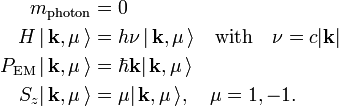
$\begin{align} m_\textrm{photon} &= 0 \\ H \,|\,\mathbf{k},\mu\,\rangle &= h\nu\, |\,\mathbf{k},\mu\,\rangle \quad \hbox{with}\quad \nu = c |\mathbf{k}| \\ P_{\textrm{EM}} \,|\,\mathbf{k},\mu\,\rangle &= \hbar\mathbf{k} |\,\mathbf{k},\mu\,\rangle \\ S_z |\,\mathbf{k},\mu\,\rangle &= \mu |\,\mathbf{k},\mu\,\rangle,\quad \mu=1,-1 .\\ \end{align}$

These equations state respectively: a photon has zero rest mass; the photon energy is hν=hc|k| (k is the wave vector, c is speed of light); its electromagnetic momentum is ℏk [ℏ=h/(2π)]; the polarization μ=±1 is the eigenvalue of the z-component of the photon spin.

[edit] Second quantization

A common way to introduce second quantization of an n particle scalar or a vector field is to start with the expansion of the field (or wave function) in a basis consisting of a complete set of functions depending on position. These expansion functions depend on the coordinate r of a single particle. The coefficients multiplying the basis functions in the expansion are interpreted as operators and (anti)commutation relations between these new operators are imposed, commutation relations for bosons and anticommutation relations for fermions (nothing happens to the basis functions themselves).

By this procedure the expanded (scalar or vector) field is converted into a fermion or boson operator field. Thus, the expansion coefficients and their complex conjugates are promoted from ordinary complex numbers to operators. It will be shown that there are two kinds: creation and annihilation operators. A creation operator creates a particle in a state described by the corresponding basis function and an annihilation operator annihilates a particle in this state.

In the case of the EM field (a vector field) A(r, t), considered below, the required expansion of the field is a Fourier expansion. A Fourier expansion is in terms of functions exp[ik⋅r]. All vector-valued expansion coefficients (also known as Fourier components of the field) have three components corresponding to the three components of the vector field A. The field A is transverse, which implies that the forward component of the expansion coefficients are zero.

[edit] Electromagnetic field and vector potential

See Fourier expansion electromagnetic field for more details.

As the term suggests, an EM field consists of two vector fields, an electric field E(r,t) and a magnetic field B(r,t). Both are time-dependent vector fields that in vacuum depend on a third vector field A(r,t) (the vector potential) through

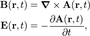
$\begin{align} \mathbf{B}(\mathbf{r}, t) &= \boldsymbol{\nabla}\times \mathbf{A}(\mathbf{r}, t)\\ \mathbf{E}(\mathbf{r}, t) &= - \frac{\partial \mathbf{A}(\mathbf{r}, t)}{\partial t}, \\ \end{align}$

here ∇×A is the curl of A. The Fourier expansion of the vector potential enclosed in a finite cubic box of volume V = L³ is (bar on top indicates complex conjugate):

$\mathbf{A}(\mathbf{r}, t) = \sum_\mathbf{k}\sum_{\mu=-1,1} \left( \mathbf{e}^{(\mu)}(\mathbf{k}) a^{(\mu)}_\mathbf{k}(t) \, e^{i\mathbf{k}\cdot\mathbf{r}} + \bar{\mathbf{e}}^{(\mu)}(\mathbf{k}) \bar{a}^{(\mu)}_\mathbf{k}(t) \, e^{-i\mathbf{k}\cdot\mathbf{r}} \right),$

where the wave vector k gives the propagation direction of the corresponding Fourier component (a polarized monochromatic wave) of A(r,t); the length of the wave vector is |k| = 2πν/c = ω/c, with ν the frequency of the mode. The components of the vector k have discrete values (a consequence of the boundary condition that A has the same value on opposite walls of the box),

$k_x = \frac{2\pi n_x}{L},\quad k_y = \frac{2\pi n_y}{L},\quad k_z = \frac{2\pi n_z}{L},\qquad n_x,\;n_y,\;n_z = 0,\, \pm1,\, \pm2,\, \ldots$

The two unit vectors e^(μ) ("polarization vectors") are perpendicular to k. They are related to the orthonormal Cartesian vectors e_x and e_y through a unitary transformation,

$\mathbf{e}^{(1)} \equiv \frac{-1}{\sqrt{2}}(\mathbf{e}_x + i \mathbf{e}_y)\quad\hbox{and}\quad\mathbf{e}^{(-1)} \equiv \frac{1}{\sqrt{2}}(\mathbf{e}_x - i \mathbf{e}_y)\quad \hbox{with}\quad \mathbf{e}_x\cdot\mathbf{k} = \mathbf{e}_y\cdot\mathbf{k} = 0.$

The k-th Fourier component of A is a vector perpendicular to k and hence is a linear combination of e⁽¹⁾ and e⁽⁻¹⁾. The superscript μ indicates a component along e^(μ). The Coulomb gauge is imposed,

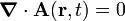
$\boldsymbol{\nabla}\cdot \mathbf{A}(\mathbf{r},t) = 0$

which makes A into a transverse field.

Clearly, the (discrete infinite) set of Fourier coefficients $a^{(\mu)}_\mathbf{k}(t)$ and $\bar{a}^{(\mu)}_\mathbf{k}(t)$ are variables defining the vector potential. In the following they will be promoted to operators with canonical commutation relations.

[edit] Quantization of EM field

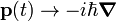
The best known example of quantization is the replacement of the time-dependent linear momentum p(t) of a particle by the rule

$\mathbf{p}(t) \rightarrow -i\hbar\boldsymbol{\nabla}$ .

Note that Planck's constant is introduced here and that the time-dependence of the classical expression is not taken over in the quantum mechanical operator (this is true in the so-called Schrödinger picture).

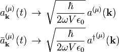
For the EM field we do something similar. The quantity ε₀ is the electric constant, which appears here because of the use of electromagnetic SI units. The quantization rules are:

$\begin{align} a^{(\mu)}_\mathbf{k}(t)\, &\rightarrow\, \sqrt{\frac{\hbar}{2 \omega V\epsilon_0}}\, a^{(\mu)}(\mathbf{k}) \\ \bar{a}^{(\mu)}_\mathbf{k}(t)\, &\rightarrow\, \sqrt{\frac{\hbar}{2 \omega V\epsilon_0}}\, {a^\dagger}^{(\mu)}(\mathbf{k}) \\ \end{align}$

subject to the boson commutation relations

$\begin{align} \big[ a^{(\mu)}(\mathbf{k}),\, a^{(\mu')}(\mathbf{k}') \big] & = 0 \\ \big[{a^\dagger}^{(\mu)}(\mathbf{k}),\, {a^\dagger}^{(\mu')}(\mathbf{k}')\big] &=0 \\ \big[a^{(\mu)}(\mathbf{k}),\,{a^\dagger}^{(\mu')}(\mathbf{k}')\big]&= \delta_{\mathbf{k},\mathbf{k}'} \delta_{\mu,\mu'}. \end{align}$

The square brackets indicate a commutator, defined by

$\big[ A, B\big] \equiv AB - BA$

for any two quantum mechanical operators A and B. The introduction of Planck's constant ℏ is essential in the transition from a classical to a quantum theory. The factor (2ωVε₀)^−½ is introduced to give the Hamiltonian (energy operator) a simple form, see below.

The quantized EM fields (operator fields) are the following

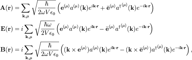
$\begin{align} \mathbf{A}(\mathbf{r}) &= \sum_{\mathbf{k},\mu} \sqrt{\frac{\hbar}{2 \omega V\epsilon_0}} \left(\mathbf{e}^{(\mu)} a^{(\mu)}(\mathbf{k}) e^{i\mathbf{k}\cdot\mathbf{r}} + \bar{\mathbf{e}}^{(\mu)} {a^\dagger}^{(\mu)}(\mathbf{k}) e^{-i\mathbf{k}\cdot\mathbf{r}} \right) \\ \mathbf{E}(\mathbf{r}) &= i\sum_{\mathbf{k},\mu} \sqrt{\frac{\hbar\omega}{2 V\epsilon_0}} \left(\mathbf{e}^{(\mu)} a^{(\mu)}(\mathbf{k}) e^{i\mathbf{k}\cdot\mathbf{r}} - \bar{\mathbf{e}}^{(\mu)} {a^\dagger}^{(\mu)}(\mathbf{k}) e^{-i\mathbf{k}\cdot\mathbf{r}} \right) \\ \mathbf{B}(\mathbf{r}) &= i\sum_{\mathbf{k},\mu} \sqrt{\frac{\hbar}{2 \omega V\epsilon_0}} \left((\mathbf{k}\times\mathbf{e}^{(\mu)}) a^{(\mu)}(\mathbf{k}) e^{i\mathbf{k}\cdot\mathbf{r}} - (\mathbf{k}\times\bar{\mathbf{e}}^{(\mu)}) {a^\dagger}^{(\mu)}(\mathbf{k}) e^{-i\mathbf{k}\cdot\mathbf{r}} \right), \\ \end{align}$

where ω = c |k| = ck = 2πc/λ and V is the volume of the box containing the field.

[edit] Hamiltonian of the field

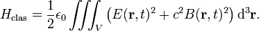
The Hamiltonian of the classical EM field is

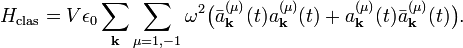
$H_{\rm clas} = \frac{1}{2}\epsilon_0\iiint_V \left( E(\mathbf{r},t)^2 + c^2 B(\mathbf{r},t)^2 \right) \mathrm{d}^3 \mathbf{r}.$

Expansion and use of the orthogonality of the Fourier basis gives

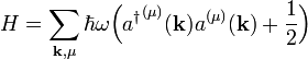
$H_{\rm clas} = V\epsilon_0 \sum_\mathbf{k}\sum_{\mu=1,-1} \omega^2 \big(\bar{a}^{(\mu)}_\mathbf{k}(t)a^{(\mu)}_\mathbf{k}(t)+ a^{(\mu)}_\mathbf{k}(t)\bar{a}^{(\mu)}_\mathbf{k}(t)\big).$

Substitution of the field operators into the classical Hamiltonian gives the Hamilton operator of the EM field,

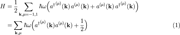
$\begin{align} H &= \frac{1}{2}\sum_{\mathbf{k},\mu=-1,1} \hbar \omega \Big({a^\dagger}^{(\mu)}(\mathbf{k})\,a^{(\mu)}(\mathbf{k}) + a^{(\mu)}(\mathbf{k})\,{a^\dagger}^{(\mu)}(\mathbf{k})\Big) \\ &= \sum_{\mathbf{k},\mu} \hbar \omega \Big({a^\dagger}^{(\mu)}(\mathbf{k})a^{(\mu)}(\mathbf{k}) + \frac{1}{2}\Big) \qquad\qquad\qquad\qquad\qquad\qquad\qquad(1) \end{align}$

By the use of the commutation relations the second line follows from the first. Note again that ℏω = hν = ℏc|k| and remember that ω depends on k, even though it is not explicit in the notation. The notation ω(k) could have been introduced, but is not common as it clutters the equations.

[edit] Digression: harmonic oscillator

The second quantized treatment of the one-dimensional quantum harmonic oscillator is a well-known topic in quantum mechanical courses. We digress and say a few words about it. The harmonic oscillator Hamiltonian has the form

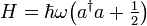
$H = \hbar \omega \big( a^\dagger a + \tfrac{1}{2} \big)$

where ω ≡ 2πν is the fundamental frequency of the oscillator. The ground state of the oscillator is designated by | 0 ⟩ and is referred to as vacuum state. It can be shown that $a^\dagger$ is an excitation operator, it excites from an n fold excited state to an n+1 fold excited state:

$a^\dagger |n \rangle = |n+1 \rangle \sqrt{n+1} \quad\hbox{in particular}\quad a^\dagger |0 \rangle = |1 \rangle \quad\hbox{and}\quad (a^\dagger)^n |0\rangle \propto |n\rangle.$

Since harmonic oscillator energies are equidistant, the n-fold excited state | n⟩ can be looked upon as a single state containing n particles (sometimes called vibrons) all of energy hν. These particles are bosons. For obvious reason the excitation operator $a^\dagger$ is called a creation operator.

From the commutation relation follows that the Hermitian adjoint $\, a$ de-excites:

$a |n \rangle = |n-1 \rangle \sqrt{n} \quad\hbox{in particular}\quad a |0 \rangle \propto 0,$

so that

$a |0 \rangle = 0.$

For obvious reason the de-excitation operator $\,a$ is called an annihilation operator.

By mathematical induction the following "differentiation rule", that will be needed later, is easily proved,

$[a, (a^\dagger)^n] = n (a^\dagger)^{n-1}\quad\hbox{with}\quad (a^\dagger)^0 = 1.$

Suppose now we have a number of non-interacting (independent) one-dimensional harmonic oscillators, each with its own fundamental frequency ω_i. Because the oscillators are independent, the Hamiltonian is a simple sum:

$H = \sum_i \hbar\omega_i \Big(a^\dagger(i) a(i) +\tfrac{1}{2} \Big).$

Making the substitution

$i \rightarrow (\mathbf{k}, \mu)$

we see that the Hamiltonian [equation (1)] of the EM field can be looked upon as a Hamiltonian of independent oscillators of energy ω = |k| c and oscillating along direction e^(μ) with μ=1,−1.

[edit] Photon states

The quantized EM field has a vacuum (no photons) state | 0 ⟩. The application to it of, say,

$\big( {a^\dagger}^{(\mu)}(\mathbf{k}) \big)^m \, \big( {a^\dagger}^{(\mu')}(\mathbf{k}') \big)^n \, \big|\,0\,\big\rangle \propto \big|(\mathbf{k},\mu)^m; \, (\mathbf{k}', \mu')^n \, \big\rangle,$

gives a quantum state of m photons in mode (k,μ) and n photons in mode (k', μ'). The proportionality symbol is used because the state on the left-hand is not normalized to unity, whereas the state on the right-hand may be normalized.

The operator

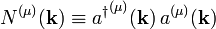
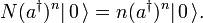
$N^{(\mu)}(\mathbf{k}) \equiv {a^\dagger}^{(\mu)}(\mathbf{k})\, a^{(\mu)}(\mathbf{k})$

is the number operator. When acting on a quantum mechanical photon state, it returns the number of photons in mode (k,μ). This also holds when the number of photons in this mode is zero, then the number operator returns zero. To show the action of the number operator on a one-photon ket, we consider

$\begin{align} N^{(\mu)}(\mathbf{k})\; |\, \mathbf{k}',\mu'\,\rangle &= {a^\dagger}^{(\mu)}(\mathbf{k})\, a^{(\mu)}(\mathbf{k})\; {a^\dagger}^{(\mu')}(\mathbf{k'})\, |\,0\,\rangle = {a^\dagger}^{(\mu)}(\mathbf{k})\,\left(\delta_{\mathbf{k},\mathbf{k'}}\delta_{\mu,\mu'} + {a^\dagger}^{(\mu')}(\mathbf{k'})\,a^{(\mu)}(\mathbf{k})\right) \, |\,0\,\rangle \\ &=\delta_{\mathbf{k},\mathbf{k'}}\delta_{\mu,\mu'} \,|\, \mathbf{k},\mu\rangle, \end{align}$

i.e., a number operator of mode (k,μ) returns zero if the mode is unoccupied and returns unity if the mode is singly occupied. To consider the action of the number operator of mode (k, μ) on a n-photon ket of the same mode, we drop the indices k and μ and consider

$N (a^\dagger)^n |\,0\,\rangle = a^\dagger \left([a, (a^\dagger)^n] + (a^\dagger)^n a\right)|0\rangle =a^\dagger\,[a, (a^\dagger)^n]\,|0\,\rangle.$

Use the "differentiation rule" introduced earlier and it follows that

$N (a^\dagger)^n |\,0\,\rangle = n (a^\dagger)^n |\,0\,\rangle.$

A photon state is an eigenstate of the number operator. This is why the formalism described here, is often referred to as the occupation number representation.

[edit] Photon energy

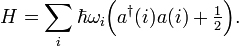
Earlier the Hamiltonian,

$H = \sum_{\mathbf{k},\mu} \hbar \omega \Big({a^\dagger}^{(\mu)}(\mathbf{k})a^{(\mu)}(\mathbf{k}) + \frac{1}{2}\Big)$

was introduced. The zero of energy can be shifted, which leads to an expression in terms of te number operator,

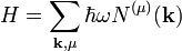
$H= \sum_{\mathbf{k},\mu} \hbar \omega N^{(\mu)}(\mathbf{k})$

The effect of H on a single-photon state is

$H|\mathbf{k},\mu\rangle \equiv H \left({a^\dagger}^{(\mu)}(\mathbf{k}) \,|0\rangle\right) = \sum_{\mathbf{k'},\mu'} \hbar\omega' N^{(\mu')}(\mathbf{k}') {a^\dagger}^{(\mu)}(\mathbf{k}) \,|\,0\,\rangle = \hbar\omega \left( {a^\dagger}^{(\mu)}(\mathbf{k}) \,|0\rangle\right) = \hbar\omega |\mathbf{k},\mu\rangle.$

Apparently, the single-photon state is an eigenstate of H and ℏω = hν is the corresponding energy. In the very same way

$H \big|(\mathbf{k},\mu)^m; \, (\mathbf{k}', \mu')^n \, \big\rangle = \left[m(\hbar\omega) + n(\hbar\omega') \right] \big|(\mathbf{k},\mu)^m; \, (\mathbf{k}', \mu')^n \, \big\rangle ,$

with

$\omega = c |\mathbf{k}|\quad\hbox{and}\quad \omega' = c |\mathbf{k}'|.$

[edit] Example photon density

In this article the electromagnetic energy density was computed that a 100kW radio station creates in its environment; at 5 km from the station it was estimated to be 2.1·10⁻¹⁰ J/m³. Is quantum mechanics needed to describe the broadcasting of this station?

The classical approximation to EM radiation is good when the number of photons is much larger than unity in the volume

$\left(\frac{\lambda}{2\pi}\right)^3 ,$

where λ is the length of the radio waves. In that case quantum fluctuations are negligible and cannot be heard.

Suppose the radio station broadcasts at ν = 100 MHz, then it is sending out photons with an energy content of νh = 1·10⁸× 6.6·10⁻³⁴ = 6.6·10⁻²⁶ J, where h is Planck's constant. The wavelength of the station is λ = c/ν = 3 m, so that λ/(2π) = 48 cm and the volume is 0.111 m³. The energy content of this volume element is 2.1·10⁻¹⁰ × 0.111 = 2.3 ·10⁻¹¹ J, which amounts to

3.5 ·10¹² photons per $\left (\frac{\lambda}{2\pi}\right)^3$

Obviously, 3.5 ·10¹² is much larger than one and hence quantum effects do not play a role; the waves emitted by this station are well into the classical limit.

[edit] Photon momentum

Introducing the Fourier expansion of the electromagnetic field into the classical form

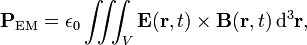
$\mathbf{P}_\textrm{EM} = \epsilon_0 \iiint_V \mathbf{E}(\mathbf{r},t)\times \mathbf{B}(\mathbf{r},t)\, \textrm{d}^3\mathbf{r},$

yields

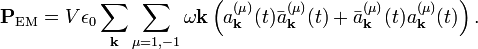
$\mathbf{P}_\textrm{EM} = V \epsilon_0 \sum_\mathbf{k}\sum_{\mu=1,-1} \omega \mathbf{k} \left( a^{(\mu)}_\mathbf{k}(t)\bar{a}^{(\mu)}_\mathbf{k}(t) + \bar{a}^{(\mu)}_\mathbf{k}(t) a^{(\mu)}_\mathbf{k}(t) \right).$

Quantization gives

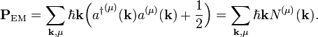
$\mathbf{P}_\textrm{EM} = \sum_{\mathbf{k},\mu} \hbar \mathbf{k} \Big({a^\dagger}^{(\mu)}(\mathbf{k})a^{(\mu)}(\mathbf{k}) + \frac{1}{2}\Big) = \sum_{\mathbf{k},\mu} \hbar \mathbf{k} N^{(\mu)}(\mathbf{k}).$

The term 1/2 could be dropped, because when one sums over the allowed k, k cancels with −k. The effect of P_EM on a single-photon state is

$\mathbf{P}_\textrm{EM} \,|\, \mathbf{k},\mu\,\rangle = \mathbf{P}_\textrm{EM} \left({a^\dagger}^{(\mu)}(\mathbf{k}) \,|0\rangle \right) = \hbar\mathbf{k} \left( {a^\dagger}^{(\mu)}(\mathbf{k}) \,|0\rangle\right)= \hbar\mathbf{k}\,|\, \mathbf{k},\mu\,\rangle .$

Apparently, the single-photon state is an eigenstate of the momentum operator, and ℏk is the eigenvalue (the momentum of a single photon).

[edit] Photon mass

The photon having non-zero linear momentum, one could imagine that it has a non-vanishing rest mass m₀, which is its mass at zero speed. However, we will now show that this is not the case: m₀ = 0.

Since the photon propagates with the speed of light, special relativity is called for. The relativistic expressions for energy and momentum squared are,

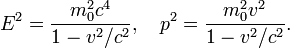
$E^2 = \frac{m_0^2 c^4}{1-v^2/c^2}, \quad p^2 = \frac{m_0^2 v^2}{1-v^2/c^2}.$

From p²/E²,

$\frac{v^2}{c^2} = \frac{c^2p^2}{E^2} \quad\Longrightarrow\quad E^2= \frac{m_0^2c^4}{1 - c^2p^2/E^2} \quad\Longrightarrow\quad m_0^2 c^4 = E^2 - c^2p^2.$

Use

$E^2 = \hbar^2 \omega^2\quad\mathrm{and}\quad p^2 = \hbar^2 k^2 = \frac{\hbar^2 \omega^2}{c^2}$

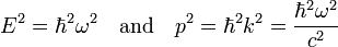
and it follows that

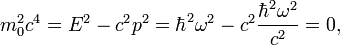
$m_0^2 c^4 = E^2 - c^2p^2 = \hbar^2 \omega^2 - c^2 \frac{\hbar^2 \omega^2}{c^2} = 0,$

so that m₀ = 0.

[edit] Photon spin

The photon can be assigned a triplet spin with spin quantum number S = 1. This is similar to, say, the nuclear spin of the ¹⁴N isotope, but with the important difference that the state with M_S = 0 is zero, only the states with M_S = ±1 are non-zero.

Define spin operators:

$S_z \equiv -i\hbar\Big( \mathbf{e}_{x}\otimes \mathbf{e}_{y} - \mathbf{e}_{y}\otimes \mathbf{e}_{x}\Big) \quad\hbox{and cyclically}\quad x\rightarrow y \rightarrow z \rightarrow x.$

The products between the two orthogonal unit vectors are dyadic products. The unit vectors are perpendicular to the propagation direction k (the direction of the z axis, which is the spin quantization axis).

The spin operators satisfy the usual angular momentum commutation relations

$[S_x, \, S_y] = i \hbar S_z \quad\hbox{and cyclically}\quad x\rightarrow y \rightarrow z \rightarrow x.$

Indeed, use the dyadic product property

$\big(\mathbf{e}_{y} \otimes \mathbf{e}_{z}\big)\;\big( \mathbf{e}_{z} \otimes \mathbf{e}_{x}\big) = (\mathbf{e}_{y}\otimes\mathbf{e}_{x})( \mathbf{e}_{z} \cdot \mathbf{e}_{z}) = \mathbf{e}_{y}\otimes\mathbf{e}_{x}$

because e_z is of unit length. In this manner,

$\begin{align} \left[S_x, \, S_y\right] &= -\hbar^2 \Big( \mathbf{e}_{y} \otimes \mathbf{e}_{z} - \mathbf{e}_{z} \otimes \mathbf{e}_{y}\Big)\; \Big( \mathbf{e}_{z} \otimes \mathbf{e}_{x} - \mathbf{e}_{x} \otimes \mathbf{e}_{z}\Big) + \hbar^2 \Big( \mathbf{e}_{z} \otimes \mathbf{e}_{x} - \mathbf{e}_{x} \otimes \mathbf{e}_{z}\Big)\; \Big( \mathbf{e}_{y} \otimes \mathbf{e}_{z} - \mathbf{e}_{z} \otimes \mathbf{e}_{y}\Big) \\ &= i\hbar \Big[ -i\hbar \big(\mathbf{e}_{x} \otimes \mathbf{e}_{y} - \mathbf{e}_{y} \otimes \mathbf{e}_{x}\big)\Big] =i\hbar S_z. \\ \end{align}$

By inspection it follows that

$-i\hbar\Big( \mathbf{e}_{x} \otimes \mathbf{e}_{y} - \mathbf{e}_{y} \otimes \mathbf{e}_{x}\Big)\cdot \mathbf{e^{(\mu)}} = \mu \mathbf{e}^{(\mu)}, \quad \mu=1,-1,$

and therefore μ labels the photon spin,

$S_z | \mathbf{k}, \mu \rangle = \mu | \mathbf{k}, \mu \rangle,\quad \mu=1,-1.$

Because the vector potential A is a transverse field, the photon has no forward (μ = 0) spin component.

[edit] References

↑ P. A. M. Dirac, The Quantum Theory of the Emission and Absorption of Radiation, Proc. Royal Soc. (London) A114, pp. 243–265, (1927) Online (pdf)
↑ The name derives from the second quantization of quantum mechanical wave functions. Such a wave function is a scalar field: the "Schrödinger field" and can be quantized in the very same way as electromagnetic fields. Since a wave function is derived from a "first" quantized Hamiltonian, the quantization of the Schrödinger field is the second time quantization is performed, hence the name.

[0] P. A. M. Dirac, The Quantum Theory of the Emission and Absorption of Radiation, Proc. Royal Soc. (London) A114, pp. 243–265, (1927) Online (pdf)

[1] The name derives from the second quantization of quantum mechanical wave functions. Such a wave function is a scalar field: the "Schrödinger field" and can be quantized in the very same way as electromagnetic fields. Since a wave function is derived from a "first" quantized Hamiltonian, the quantization of the Schrödinger field is the second time quantization is performed, hence the name.

[1]

[2]

Quantization of the electromagnetic field

Contents

[edit] Introduction

[edit] Second quantization

[edit] Electromagnetic field and vector potential

[edit] Quantization of EM field

[edit] Hamiltonian of the field

[edit] Digression: harmonic oscillator

[edit] Photon states

[edit] Photon energy

[edit] Example photon density

[edit] Photon momentum

[edit] Photon mass

[edit] Photon spin

[edit] References

Personal tools

Namespaces

Variants

Views

Actions

Search

Navigation

Community

Toolbox