Maxwell equations

In physics, the Maxwell equations are the mathematical equations that describe how electric and magnetic fields are created by electric charges and electric currents and in addition they give relationships between these fields. The equations are named after the Scottish physicist James Clerk Maxwell, who published them (in a somewhat old-fashioned notation) in 1865.[1] The Maxwell equations are still considered to be valid, even in quantum electrodynamics where the electromagnetic fields are reinterpreted as quantum mechanical operators satisfying canonical commutation relations, see the article quantization of the electromagnetic field.
Among physicists, the Maxwell equations take a place of importance equal to Newton's equation F=ma, Einstein's equation E=mc2, and Schrödinger's equation Hψ=Eψ. Yet, among the general, well-educated, public, Clerk Maxwell does not have the same fame as the other three physicists. This is somewhat surprising, because the applications of Maxwell's equations have far-reaching impact on society. Maxwell was the first to see that his equations predict the existence of electromagnetic waves. Without knowledge and understanding of these waves we would not have radio, radar, television, cell phones, global positioning systems, etc. Maybe, the lack of fame of Maxwell's equations is due to the fact that they cannot be caught in a simple iconic equation like E=mc2. In modern textbooks Maxwell's equations are presented as four fairly elaborate vector equations, involving abstract mathematical notions as curl and divergence.[2]
There are two sets of Maxwell's equations, the most basic ones are the microscopic equations, which describe the electric field E and the magnetic field B in vacuo, together with their sources (charge- and current-densities). That is, it is assumed that there is no other matter in the system than the charges and currents accounted for in the equations; the charges and currents are located in empty space.
The other set is known as the macroscopic equations. Here it is assumed that, instead of the vacuum, there is a continuous medium present[3] (air, for instance) that is polarizable and magnetizable. In this case two additional vectors, P (the polarization vector of the medium) and M (the magnetization vector of the medium) play a role. It will be discussed below that it is convenient to replace those two vectors by two auxiliary vectors, the electric displacement D and the magnetic field H.[4] The Dutch physicist Lorentz showed in the 1890s that the macroscopic equations can be derived from the microscopic equations by an averaging of electric and magnetic dipoles over the medium. In that sense the microscopic equations are the most basic. On the other hand, given the macroscopic equations, one simply retrieves the microscopic equations by putting P = M = 0.
It is generally assumed that the Maxwell equations, together with the Lorentz force and Newton's second law, determine completely the classical, i.e., non-quantum, behavior of a system of moving electric charges. However, their solution is in general very difficult and requires some sort of iterative procedure, because moving charges generate fields (electric as well as magnetic) and these fields give a Lorentz force that acting on the charges, through Newton's equation changes the motion of the charges. The changed motion gives different fields and a new Lorentz force that acts differently on the charges, and so on.
| See for the physical background and more explanation of the Maxwell equations, respectively, |
| * Gauss′ law (no magnetic monopoles) |
| * Faraday's law (electromagnetism) (voltage generated by change in magnetic induction) |
| * Gauss′ law (electrostatic field from charge density) |
| * Ampère's law (magnetic field generated by current) |
[edit] Microscopic equations
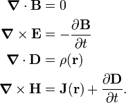
The vector fields E and B depend on time t and position r, for brevity this dependence is not shown explicitly in the equations. The first two Maxwell equations do not depend on charges or currents. In SI units they read,
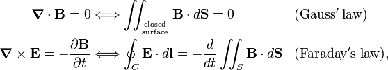
where ∇• stands for the divergence of a vector field and ∇× for its curl.
The first Maxwell equation, given in differential form, is converted to the magnetic Gauss law, an integral equation, by integrating over a volume V and applying the divergence theorem. The closed surface integrated over is the surface enveloping V. The second Maxwell equation is converted into Faraday's law by integrating left- and right-hand side over a surface S bounded by a contour C and applying Stokes' theorem.
Let ρ(r) be an electric charge density (charge per unit volume) and J(r) be an electric current density (electric current per unit area), both quantities enter the second set of Maxwell equations (again in SI units)
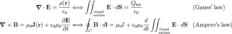
The third Maxwell equation is converted to the electrostatic Gauss law by integrating over a volume V and applying the divergence theorem. The closed surface integrated over is the surface enveloping V; Qtot is the total electric charge contained in V. The fourth Maxwell equation is converted into Ampère's law by integrating left- and right-hand side over a surface S bounded by a contour C and applying Stokes' theorem. Here we need to add the historical note that A.-M. Ampère had not seen the necessity of the second term on the right-hand side containing the time derivative of the electric field, the so-called displacement current. Ampère formulated his law for the conduction current I only, which is correct if the displacement current is zero. It was J. Clerk Maxwell who recognized the need of the displacement current.
The electric constant ε0 and the magnetic constant μ0 are peculiar to the use of SI units. Their product satisfies

where c is the speed of light.
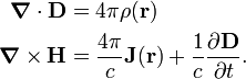
The microscopic Maxwell equations in Gaussian units do not contain the electric and magnetic constant, but c instead, they read
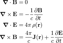
The factor 4π arises here because the Gaussian system of units is not rationalized, in contrast to the SI system.
[edit] Macroscopic equations
In SI units the electric displacement D and the magnetic field H are defined by the relations:
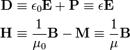
where P is the polarization and M is the magnetization of the medium. The relations between the fields that contain the material properties relative permittivity ε (formerly known as dielectric constant) and magnetic susceptibility μ are known as constitutive relations. The somewhat asymmetric definition of the electric and magnetic auxiliary fields D and H has a historical origin. For many years the field H was seen as the analogue of E and B was seen as an auxiliary field, analogous to D. Later, when it became clear that there are no magnetic charges and currents, the field B was considered to be the basic field. The same historic circumstance explains that B is usually called magnetic induction and H magnetic field.
The first two macroscopic Maxwell equations (the ones that do not contain charge and current densities) are exactly the same as the corresponding microscopic (vacuum) equations, the other two equations are very similar but are in terms of the auxiliary fields,
Some textbooks introduce the auxiliary fields D and H also for the vacuum (the microscopic case). They follow easily from the defining equations by putting P = M = 0. Clearly, in the vacuum D is almost equal to E and H to B, so that there is no good reason to introduce these fields for the vacuum.
In Gaussian units the auxiliary fields in vacuum are identical to the basic fields, because in Gaussian units D and H are defined as

so that in vacuum indeed D ≡ E and H ≡ B. The second set of Maxwell equations in Gaussian units is as follows,
[edit] Brief history
By Maxwell's own words, his mathematical work is a translation of Michael Faraday's earlier qualitative ideas about lines of force; however, this statement gives too much credit to Faraday. The first to cast some of Faraday's ideas in mathematical form was the British physicist William Thomson (the later Lord Kelvin). Also André-Marie Ampère in France and Carl Friedrich Gauss in Germany were very influential for Maxwell's work.
Two of Maxwell's own most important—and for some time controversial—contributions to the theory of electromagnetism were the displacement current and the theoretical discovery of electromagnetic waves. Maxwell's suggestion that ordinary visible light is an electromagnetic wave is one of the milestones in the history of science. This observation unified the fields of electromagnetism and optics, which were unrelated until then. Maxwell came to this suggestion by noticing that the speed of propagation of electromagnetic waves was very close to the speed of light. He wrote:
- This velocity is so nearly that of light, that it seem we have strong reason to conclude that light itself (including radiant heat, and other radiations if any) is an electromagnetic disturbance in the form of waves propagated through the electromagnetic field according to electromagnetic laws.
This statement, written in 1865, remained controversial until 1886 when Heinrich Hertz, then in Karlsruhe, was able to generate and detect electromagnetic waves in the laboratory. Before that, Hertz had studied and rederived Maxwell's equations, as had Oliver Heaviside in England. The latter, who is one of the fathers of vector analysis, had cast the equations in the vector form given above (four vector equations). Maxwell himself had formulated his theory in terms of twenty scalar equations.
It seems likely that neither Maxwell nor Hertz recognized the importance of their discoveries for communications. It was only in the 1890s, when Maxwell's theory was completely accepted due to the work by Lorentz, George Francis FitzGerald, and others, that the Italian engineer Guglielmo Marconi started to experiment with wireless telegraphy.
[edit] References
- ↑ J. Clerk Maxwell, A Dynamical Theory of the Electromagnetic Field, Phil. Trans. Roy. Soc., vol. 155, pp. 459 - 512 (1865) online
- ↑ Of course, Hψ=Eψ may look simple, but this is deceptive, the equation, written out in full, is at least as complicated as Maxwell's equations.
- ↑ It is known that matter is not continuous, but consists of particles, atoms and molecules. However, these are so small that there is a regime of magnitude where it is not contradictory to consider infinitesimal volume elements of the continuous medium. Classical electrodynamics shares this view of matter with classical aerodynamics and hydrodynamics and many other engineering sciences.
- ↑ It is somewhat unfortunate that both B and H are referred to as "magnetic field". Therefore B is often called magnetic induction or magnetic flux density.