Quantum computation

Throughout this article the Many Worlds Interpretation (MWI) of quantum mechanics is used.
Contents |
[edit] Differences with classical computation
In classical computation there is the concept of a discrete bit, taking only one of two values. However , the world which classical physics describes is that of continua. Thus this is obviously not an ideal way of attempting to describe or simulate the world in which we live. Feynman was the first to consider the idea of a quantum computer being necessary to simulate the quantum mechanical world in which we live.[1]
[edit] Quantum computers and information theory
The quantum mechanical analogue of the classical bit is the qubit. A qubit is an actual physical system, all of whose observables are Boolean.
[edit] Interference & a simple computation
[edit] Quantum algorithms
An algorithm is a hardware-independent recipe for performing a particular computation. A program is a way of preparing a specific computer to do such a task. Algorithms for quantum computers offer a wider range of computational tasks which may be solved by the use of interference. Some of the new possibilities which are opened up may prove to have drastic consequences for the future: e.g. Shor's algorithm relevance to cryptography.
[edit] Oracles
An oracle is a black box which it is impossible to look inside and performs a particular function f on the input qubits in a time which is independent of the particular input. It is not possible.
They are used to simplify the analysis of algorithms as the specific nature of how a task is performed is irrelevant due to the criterion of hardware-independence. The oracle must of course be reversible as the laws of QM do not make a distinction between forwards and backwards time (i.e. time does not have 'an arrow').
[edit] Dynamics of quantum gates in Schrödinger picture
NB In the Schrödinger picture the state vector evolves in the following manner:

where U is the characteristic unitary matrix of the gate.
[edit] NOT

So if  then
then 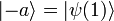
[edit] Controlled Not, CNOT
This i a two input gate where whether the NOT operation is performed on the second is dependant (i.e. controlled) by the value of the first input bit which is unchanged.

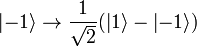
[edit] Hadamard gate, H
The Hadamard gate, normally denoted as H, creates an equally weighted superposition of the  and
and  states. There is no classical analogue of it.
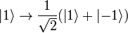
H2 = I i.e the Hadamard gate is self-inverse.
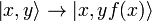
[edit] Oracle
An oracle which performs the function f(x) has the following dynamics in the Schrödinger picture. The value of y is normally set to one so that the output is x and f(x).
[edit] Deutsch algorithm
Let us create an oracle which performs the following function: 
There are four possibilities for this function:
- identity:

- not:

- output -1:

- output 1:

Computational task: To determine if f(1) = f( − 1).
This is equivalent to trying to determine f(1)f( − 1) without looking inside the oracle above.
Classically this may be done by consulting the oracle twice. [diagram of classical situation] However, using quantum computation the oracle need only be consulted once.
(N.B. For the analysis of algorithms, the Schrödinger picture is often preferable and thus shall be used here. It is of course still possible to use the Heisenberg picture.


Now we must examine the two possibilities 1) f(1) = f( − 1) and 2) f(1) = − f( − 1)
1. Let f(1) = f( − 1) = f

2. Let f(1) = − f( − 1) = f
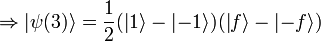
In each of these cases the state vector when t=3 is a superposition of two pure states: 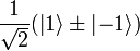 and
and 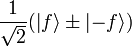 . The purpose of the final Hadamard gate is to differentiate between the states and thus determine whether f(1) = f( − 1) or not.
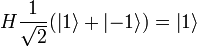
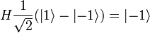
Thus 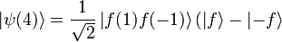
[edit] Grover's algorithm
[edit] Shor's algorithm
Shor's algorithm is used to find the factors of a number. It is particularly important because of the use in cryptography of multiplying together two large prime numbers. Factoring this number into its prime factors allows the cracking of the code.
The algorithm itself has two parts: one quantum and one classical. The latter can be done in O(xn) time. The use of a quantum algorithm makes this true for the former part as well.
Let us wish to factor a number n. The first part of the algorithm wishes to find the period, r, of the function:
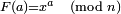 , i.e. find r such that
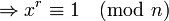
Once r has been found by use of quantum parallelism, the second part of the algorithm may be performed:
- x0(mod n) = 1
-
 etc.
etc.

-
 if r is even.
[edit] References
Based on a talk given by Charles Blackham to 6P at Winchester College, UK on 7/3/07
- Lectures on Quantum Computation by David Deutsch
- Cambridge Centre for Quantum Computation
- ↑ R.P. Feynman International Journal of Theoretical Physics 21(6/7) 1982
| |
Some content on this page may previously have appeared on Citizendium. |