Harmonic oscillator (quantum)

The prototype of a one-dimensional harmonic oscillator is a mass m vibrating back and forth on a line around an equilibrium position. In quantum mechanics, the one-dimensional harmonic oscillator is one of the few systems that can be treated exactly, i.e., its Schrödinger equation can be solved analytically.
Although the harmonic oscillator per se is not very important, a large number of systems are governed approximately by the harmonic oscillator equation. Whenever one studies the behavior of a physical system in the neighborhood of a stable equilibrium position, one arrives at equations which, in the limit of small oscillations, are those of a harmonic oscillator. Two well-known examples are the vibrations of the atoms in a diatomic molecule about their equilibrium position and the oscillations of atoms or ions of a crystalline lattice. Also the energy of electromagnetic waves in a cavity can be looked upon as the energy of a large set of harmonic oscillators.
[edit] Lowest wave functions
The characterizing feature of the one-dimensional harmonic oscillator is a parabolic potential field that has a single minimum usually referred to as the "bottom of the potential well". As stated above, the Schrödinger equation of the one-dimensional quantum harmonic oscillator can be solved exactly, yielding analytic forms of the wave functions (eigenfunctions of the energy operator). The corresponding energy eigenvalues are labeled by a single quantum number n,

where h is Planck's constant and ν depends on the the mass and the stiffness of the oscillator (see below). Note that for n = 0 the energy E0 is not equal to zero, but equal to the zero-point energy ½hν. This well-defined, non-vanishing, zero-point energy is due to the fact that the position x of the oscillating particle cannot be sharp (have a single value), since the operator x does not commute with the energy operator. Hence, by Heisenberg's uncertainty relation, energy and position cannot be sharp simultaneously. Classically, the oscillating particle can come to rest at the bottom of the potential well, where it has zero kinetic and potential energy and a well-defined—sharp—position. Quantum mechanically this is not possible, the position x of the particle of lowest possible energy is described by a wave function (a Gaussian function) of energy ½hν.
The four lowest energy harmonic oscillator eigenfunctions are shown in the figure. Note that the lowest function (blue) has indeed the form of a Gaussian function. The functions are shifted upward such that their energy eigenvalues coincide with the asymptotic levels, the zero levels of the wave functions at x = ±∞. As an example of a zero level, the zero (asymptotic) energy of the n = 2 function (black) is plotted as the black horizontal line of constant energy
- E2 = (2+ ½) hν = 5 hν/2 ≡ 5/2 ℏ ω.
According to quantum mechanics, the wave function squared of a point mass, |ψ(x)|², is the probability of finding the mass in the point x. In the figure we see that the probability of finding the oscillating mass at points to the left (for negative x) or to the right (for positive x) of V(x) is non-zero and we notice that for these points the potential energy V(x) is larger than the energy eigenvalue. As an example two small vertical lines are plotted: to the left of the small line that lies at negative x the potential energy is larger than E2, the energy of the n = 2 level. The same holds for the region to the right of the small black line at positive x. Note that the n = 2 wave function (black) is not zero in these regions.
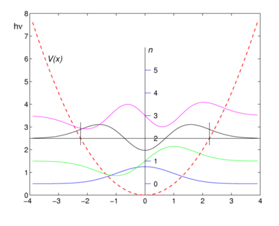
In classical mechanics the potential energy V can never surpass the total energy E, because V = E − T and the classical kinetic energy T is non-negative, so that V ≤ E. This is why the region, where the energy eigenvalue of an eigenfunction is smaller than the potential energy, is called a classically forbidden region. The fact that the probability of finding a mass in a classically forbidden is non-zero, is often expressed by stating that the point mass can tunnel into the potential wall. This tunnel effect is one of the more intriguing aspects of quantum mechanics.
[edit] Schrödinger equation
The time-independent Schrödinger equation of the harmonic oscillator has the form
![\left[-\frac{\hbar^2}{2m}\frac{\mathrm{d}^2}{\mathrm{d}x^2} + \frac{1}{2}k x^2\right] \psi = E\psi](../w/images/math/4/8/6/486b0e8254b4daad6f2ee3d657e869c4.png)
The two terms between square brackets are the Hamiltonian (energy operator) of the system: the first term is the kinetic energy operator and the second the potential energy operator. The quantity ℏ is Planck's reduced constant, m is the mass of the oscillator, and k is Hooke's spring constant describing the stiffness of the oscillator. See the classical harmonic oscillator for further explanation of m and k.
The solutions of the Schrödinger equation are characterized by a vibration quantum number n = 0,1,2, … and are of the form
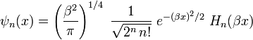
with

Here
The functions Hn(x) are Hermite polynomials; the first few are:

The graphs of the first four eigenfunctions are shown in the figure. Note that the functions of even n are even, that is,  , while those of odd n are antisymmetric
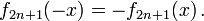
[edit] Solution of the Schrödinger equation
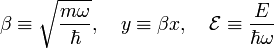
We rewrite the Schrödinger equation in order to hide the physical constants m, k, and h. As a first step we define the angular frequency ω ≡ √k/m, the same formula as for the classical harmonic oscillator:
![\frac{1}{2}\left[-\frac{\hbar^2}{m}\frac{\mathrm{d}^2}{\mathrm{d}x^2} + m\omega^2 x^2\right] \psi = E\psi.](../w/images/math/8/8/c/88cc1dc447338987693b7e89489434b5.png)
Secondly, we divide through by  , a factor that has dimension energy,
![\frac{1}{2}\left[-\frac{\hbar}{m\omega}\frac{\mathrm{d}^2}{\mathrm{d}x^2} + \frac{m\omega}{\hbar} x^2\right] \psi = \frac{E}{\hbar\omega}\psi.](../w/images/math/d/e/9/de9d7152a88429695826ce085174071a.png)
Write
and the Schrödinger equation becomes
![\frac{1}{2}\left[- \frac{1}{\beta^2}\frac{\mathrm{d}^2}{\mathrm{d}x^2} + \beta^2 x^2\right] \psi = \mathcal{E}\psi\quad \Longrightarrow\quad \frac{1}{2}\left[-\frac{\mathrm{d}^2}{\mathrm{d}y^2} + y^2\right] \psi = \mathcal{E} \psi.](../w/images/math/a/2/0/a205c0d612d531eb9edbbe17a1298960.png)
Note that all constants are hidden in the equation on the right.
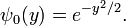
A particular solution of this equation is
We verify this
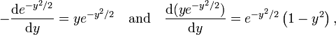
so that
![\frac{1}{2}\left[-\frac{\mathrm{d}^2}{\mathrm{d}y^2} + y^2\right] e^{-y^2/2} = \frac{1}{2}\left[e^{-y^2/2}\left(1 - y^2\right) + y^2 e^{-y^2/2}\right] = \frac{1}{2} e^{-y^2/2}.](../w/images/math/7/f/0/7f006e28c1d607b6373fce8d1fff9a80.png)
We conclude that ψ0(y) ≡ exp(-y2/2) is an eigenfunction
![\frac{1}{2}\left[-\frac{\mathrm{d}^2}{\mathrm{d}y^2} + y^2\right] \psi_0 = \frac{1}{2} \psi_0,](../w/images/math/9/5/0/950cf6675ee4518535017550ba990ef5.png)
with eigenvalue
This encourages us to try to find a total solution ψ(y) by a function of the form

Use the Leibniz rule
and
![\frac{1}{2} \left[- \frac{d^2 \psi_0} {dy^2} + y^2 \psi_0\right] f = \frac{1}{2}\psi_0 f \quad \hbox{and} \quad \frac{d \psi_0}{dy} = - y\psi_0](../w/images/math/3/1/2/312be6c3b502daec7630972c7548157c.png)
then we see
![\frac{1}{2}\left[- \frac{d^2 (\psi_0 f)}{dy^2} +y^2 \psi_0 f \right] = \frac{1}{2}\psi_0 f +y\psi_0\frac{df}{dy} - \frac{1}{2}\frac{d^2 f} {dy^2}\psi_0 = \mathcal{E} \psi_0 f.](../w/images/math/a/1/c/a1c9e9f2204c18e16d6f80bf801f8a75.png)
Divide through by −ψ0(y)/2 and we find the equation for f
The differential equation of Hermite with polynomial solutions Hn(y) is
Due to the appearance of the integer coefficient 2n in the last term the solutions are polynomials. We see that if we put

that we have solved the Schrödinger equation for the harmonic oscillator. The unnormalized solutions are
