Rotation matrix

From Knowino

Jump to: navigation, search

In mathematics and physics a rotation matrix is synonymous with a 3×3 orthogonal matrix, which is a real 3×3 matrix R satisfying

$\mathbf{R}^\mathrm{T} = \mathbf{R}^{-1},$

where T stands for the transposed matrix and R⁻¹ is the inverse of R.

1 Connection of an orthogonal matrix to a rotation
2 Properties of an orthogonal matrix
- 2.1 Compact notation
3 Explicit expression of rotation operator
4 Explicit expression of rotation matrix
5 Vector rotation
- 5.1 Case that "from" and "to" vectors are anti-parallel
6 Change of rotation axis
7 References

Connection of an orthogonal matrix to a rotation

In general a motion of a rigid body (which is equivalent to an angle and distance preserving transformation of affine space) can be described as a translation of the body followed by a rotation. By a translation all points of the body are displaced, while under a rotation at least one point of the body stays in place. Let the the fixed point be O. By Euler's theorem follows that then not only the point is fixed but also an axis—the rotation axis— through the fixed point. Write $\hat{n}$ for the unit vector along the rotation axis and φ for the angle over which the body is rotated, then the rotation operator on ℝ³ is written as ℛ(φ, n̂).

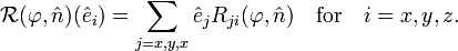
Erect three Cartesian coordinate axes with the origin in the fixed point O and take unit vectors $\hat{e}_x,\;\hat{e}_y,\;\hat{e}_z$ along the axes, then the 3×3 rotation matrix $\mathbf{R}(\varphi, \hat{n})$ is defined by its elements $R_{ji}(\varphi, \hat{n})$ :

$\mathcal{R}(\varphi, \hat{n})(\hat{e}_i) = \sum_{j=x,y,x} \hat{e}_j R_{ji}(\varphi, \hat{n}) \quad\hbox{for}\quad i=x,y,z.$

In a more condensed notation this equation can be written as

$\mathcal{R}(\varphi, \hat{n})\left(\hat{e}_x,\;\hat{e}_y,\;\hat{e}_z\right) = \left(\hat{e}_x,\;\hat{e}_y,\;\hat{e}_z\right) \; \mathbf{R}(\varphi, \hat{n}).$

Given a basis of the linear space ℝ³, the association between a linear map and its matrix is one-to-one.

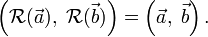
A rotation $\mathcal{R}$ (for convenience sake the rotation axis and angle are suppressed in the notation) leaves the shape of a rotated rigid body intact, so that all distances within the body are invariant. If the body is 3-dimensional—it contains three linearly independent vectors with origins in the invariant point—it holds that for any pair of vectors $\vec{a}$ and $\vec{b}$ in ℝ³ the inner product is invariant, that is,

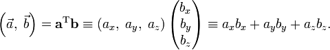
$\left(\mathcal{R}(\vec{a}),\;\mathcal{R}(\vec{b}) \right) = \left(\vec{a},\;\vec{b}\right).$

A linear map with this property is called orthogonal. It is easily shown that a similar vector-matrix relation holds. First we define column vectors (stacked triplets of real numbers given in bold face):

$\vec{a} =\left(\hat{e}_x,\;\hat{e}_y,\;\hat{e}_z\right)\begin{pmatrix}a_x\\a_y\\a_z\end{pmatrix} \;\stackrel{\mathrm{def}}{=}\; \left(\hat{e}_x,\;\hat{e}_y,\;\hat{e}_z\right) \mathbf{a} \quad\hbox{and}\quad \vec{b} =\left(\hat{e}_x,\;\hat{e}_y,\;\hat{e}_z\right)\begin{pmatrix}b_x\\b_y\\b_z\end{pmatrix} \;\stackrel{\mathrm{def}}{=}\; \left(\hat{e}_x,\;\hat{e}_y,\;\hat{e}_z\right) \mathbf{b}$

and observe that the inner product becomes by virtue of the orthonormality of the basis vectors

$\left( \vec{a},\; \vec{b} \right) = \mathbf{a}^\mathrm{T} \mathbf{b}\equiv \left(a_x,\;a_y,\;a_z\right) \begin{pmatrix}b_x\\b_y\\b_z\end{pmatrix} \equiv a_xb_x+a_yb_y+a_zb_z.$

The invariance of the inner product under the rotation operator $\mathcal{R}$ leads to

$\mathbf{a}^\mathrm{T}\; \mathbf{b} =\big(\mathbf{R}\mathbf{a}\big)^\mathrm{T}\; \mathbf{R}\mathbf{b} = \mathbf{a}^\mathrm{T} \mathbf{R}^\mathrm{T}\; \mathbf{R}\mathbf{b},$

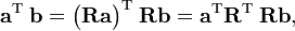
since this holds for any pair a and b it follows that a rotation matrix satisfies

$\mathbf{R}^\mathrm{T} \mathbf{R} = \mathbf{E},$

where E is the 3×3 identity matrix. For finite-dimensional matrices one shows easily

$\mathbf{R}^\mathrm{T} \mathbf{R} = \mathbf{E} \quad \Longleftrightarrow\quad\mathbf{R}\mathbf{R}^\mathrm{T} = \mathbf{E}.$

A matrix with this property is called orthogonal. So, a rotation gives rise to a unique orthogonal matrix.

Conversely, consider an arbitrary point P in the body and let the vector $\overrightarrow{OP}$ connect the fixed point O with P. Expressing this vector with respect to a Cartesian frame in O gives the column vector p (three stacked real numbers). Multiply p by the orthogonal matrix R, then p′ = Rp represents the rotated point P′ (or, more precisely, the vector $\overrightarrow{OP'}$ is represented by column vector p′ with respect to the same Cartesian frame). If we map all points P of the body by the same matrix R in this manner, we have rotated the body. Thus, an orthogonal matrix leads to a unique rotation.

Note that the Cartesian frame is fixed here and that points of the body are rotated, this is known as an active rotation. Instead, the rigid body could have been left invariant and the Cartesian frame could have been rotated, this also leads to new column vectors of the form p′ ≡ Rp, such rotations are referred to as passive.

Properties of an orthogonal matrix

Writing out matrix products it follows that both the rows and the columns of the matrix are orthonormal (normalized and orthogonal). Indeed,

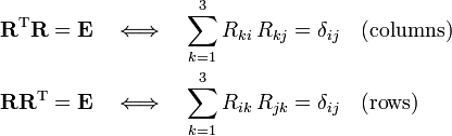
$\begin{align} \mathbf{R}^\mathrm{T} \mathbf{R} &= \mathbf{E} \quad\Longleftrightarrow\quad \sum_{k=1}^{3} R_{ki}\, R_{kj} =\delta_{ij} \quad\hbox{(columns)} \\ \mathbf{R} \mathbf{R}^\mathrm{T} &= \mathbf{E} \quad\Longleftrightarrow\quad \sum_{k=1}^{3} R_{ik}\, R_{jk} =\delta_{ij} \quad\hbox{(rows)} \\ \end{align}$

where δ_ij is the Kronecker delta.

Orthogonal matrices come in two flavors: proper (det = 1) and improper (det = −1) rotations. Indeed, invoking some properties of determinants, one can prove

$1=\det(\mathbf{E})=\det(\mathbf{R}^\mathrm{T}\mathbf{R}) = \det(\mathbf{R}^\mathrm{T})\det(\mathbf{R}) = \det(\mathbf{R})^2 \quad\Longrightarrow \quad \det(\mathbf{R}) = \pm 1.$

Compact notation

A compact way of presenting the same results is the following. Designate the columns of R by r₁, r₂, r₃, i.e.,

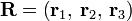$\mathbf{R} = \left(\mathbf{r}_1,\, \mathbf{r}_2,\, \mathbf{r}_3 \right)$ .

The matrix R is orthogonal if

$\mathbf{r}_i^\mathrm{T} \mathbf{r}_j \equiv \mathbf{r}_i \cdot \mathbf{r}_j = \delta_{ij}, \quad i,j = 1,2,3 .$

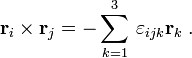
The matrix R is a proper rotation matrix, if it is orthogonal and if r₁, r₂, r₃ form a right-handed set, i.e.,

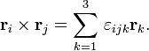
$\mathbf{r}_i \times \mathbf{r}_j = \sum_{k=1}^3 \, \varepsilon_{ijk} \mathbf{r}_k .$

Here the symbol × indicates a cross product and $\varepsilon_{ijk}$ is the antisymmetric Levi-Civita symbol,

$\begin{align} \varepsilon_{123} =&\; \varepsilon_{312} = \varepsilon_{231} = 1 \\ \varepsilon_{213} =&\; \varepsilon_{321} = \varepsilon_{132} = -1 \end{align}$

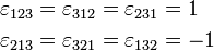
and $\varepsilon_{ijk} = 0$ if two or more indices are equal.

The matrix R is an improper rotation matrix if its column vectors form a left-handed set, i.e.,

$\mathbf{r}_i \times \mathbf{r}_j = - \sum_{k=1}^3 \, \varepsilon_{ijk} \mathbf{r}_k \; .$

The last two equations can be condensed into one equation

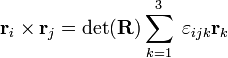
$\mathbf{r}_i \times \mathbf{r}_j = \det(\mathbf{R}) \sum_{k=1}^3 \; \varepsilon_{ijk} \mathbf{r}_k$

by virtue of the the fact that the determinant of a proper rotation matrix is 1 and of an improper rotation −1. This was proved above, an alternative proof is the following: The determinant of a 3×3 matrix with column vectors a, b, and c can be written as scalar triple product

$\det\left(\mathbf{a},\,\mathbf{b},\, \mathbf{c}\right) = \mathbf{a} \cdot (\mathbf{b}\times\mathbf{c})$ .

It was just shown that for a proper rotation the columns of R are orthonormal and satisfy,

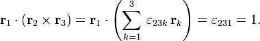
$\mathbf{r}_1 \cdot (\mathbf{r}_2 \times \mathbf{r}_3 ) = \mathbf{r}_1 \cdot\left(\sum_{k=1}^3 \, \varepsilon_{23k} \, \mathbf{r}_k \right) = \varepsilon_{231} = 1 .$

Likewise the determinant is −1 for an improper rotation.

Explicit expression of rotation operator

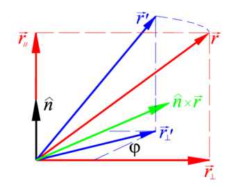
Rotation of vector $\scriptstyle \vec{r}$ around n̂ over φ.
(i) The red vectors and black axis n̂ are in the plane of the screen.
(ii) The blue vectors are obtained by rotation into the screen.
(iii) The green cross product in x-y plane is perpendicular to the screen, pointing away from the reader.

Let $\overrightarrow{OP} \equiv \vec{r}$ be a vector pointing from the fixed point O of a rigid body to an arbitrary point P of the body. A rotation of this arbitrary vector around the unit vector n̂ over an angle φ can be written as

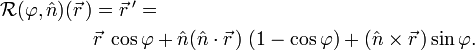
$\begin{align} \mathcal{R}(\varphi, \hat{n})(\vec{r}\,)&= \vec{r}\,' = \\ & \vec{r}\;\cos\varphi + \hat{n} (\hat{n}\cdot\vec{r}\,)\; (1- \cos\varphi) + (\hat{n} \times \vec{r}\,) \sin\varphi . \\ \end{align}$

where • indicates an inner product and the symbol × a cross product.

It is easy to derive this result. Indeed, decompose the vector to be rotated into two components, one along the rotation axis and one perpendicular to it (see the figure on the right)

$\vec{r} = \vec{r}_\parallel + \vec{r}_\perp\quad\hbox{with}\quad \vec{r}_\parallel = \hat{n} (\hat{n}\cdot\vec{r}\,),$

and

$\vec{r}_\perp = \vec{r} - \vec{r}_\parallel =\vec{r}- \hat{n} (\hat{n}\cdot\vec{r}\,),$

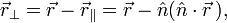
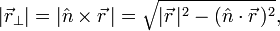
so that, in view of |n̂| = 1,

$|\vec{r}_\perp|^2 = r^2 - (\hat{n}\cdot\vec{r}\,)^2$

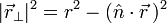
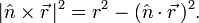
and from |a×b|² = a²b² − (a⋅b)² follows

$|\hat{n} \times \vec{r}\,|^2 = r^2 - (\hat{n}\cdot\vec{r}\,)^2.$

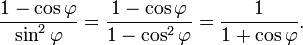
Upon rotation, the component of the rotated vector along the rotation axis is invariant, only its component orthogonal to the rotation axis changes. By virtue of the following fact (in words: length of basis vector along x-axis is length of basis vector along y-axis):

$|\vec{r}_\perp| = |\hat{n} \times \vec{r}\,| = \sqrt{|\vec{r}\,|^2 - (\hat{n}\cdot\vec{r}\,)^2},$

the rotation property simply is

$\vec{r}_\perp \mapsto \vec{r}\,'_\perp = \cos\varphi\;\vec{r}_\perp + \sin\varphi\;(\hat{n}\times\vec{r}\,).$

Hence

$\vec{r}\,' = \hat{n} (\hat{n}\cdot\vec{r}\,) + \left[\vec{r}- (\hat{n}\cdot\vec{r}\,) \hat{n}\right]\cos\varphi+(\hat{n}\times\vec{r}\,)\sin\varphi.$

Some reshuffling of the terms gives the required result.

Explicit expression of rotation matrix

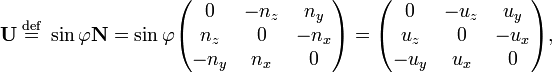
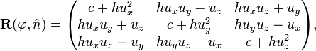
It will be shown that

$\mathbf{R}(\varphi, \hat{n}) = \mathbf{E} + \sin\varphi \mathbf{N} +(1-\cos\varphi)\mathbf{N}^2,$

where (see cross product for more details)

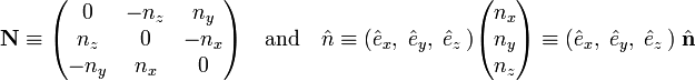
$\mathbf{N} \equiv \begin{pmatrix} 0 & -n_z & n_y \\ n_z& 0 & -n_x \\ -n_y& n_x & 0 \end{pmatrix}\quad\hbox{and}\quad \hat{n} \equiv (\hat{e}_x,\;\hat{e}_y,\;\hat{e}_z\,) \begin{pmatrix} n_x \\ n_y \\ n_z \\ \end{pmatrix} \equiv (\hat{e}_x,\;\hat{e}_y,\;\hat{e}_z\,) \; \hat{\mathbf{n}}$

Note further that the dyadic product satisfies (as can be shown by squaring N),

$\hat{\mathbf{n}}\otimes\hat{\mathbf{n}} = \mathbf{N}^2 + \mathbf{E}, \quad\hbox{with}\quad |\hat{\mathbf{n}}| = 1$

and that

$\hat{n} (\hat{n}\cdot\vec{r}\,) \leftrightarrow (\hat{\mathbf{n}}\otimes\hat{\mathbf{n}})\;\mathbf{r} = \left(\mathbf{N}^2 + \mathbf{E}\right) \mathbf{r}.$

Translating the result of the previous section to coordinate vectors and substituting these results gives

$\begin{align} \mathbf{r}' &= \left[\cos\varphi\; \mathbf{E} +(1-\cos\varphi)(\mathbf{N}^2 + \mathbf{E}) + \sin\varphi \mathbf{N} \right] \mathbf{r} \\ &= \left[\mathbf{E} + (1-\cos\varphi) \mathbf{N}^2 + \sin\varphi \mathbf{N}\right] \mathbf{r}, \qquad\qquad\qquad\qquad\qquad(1) \end{align}$

which gives the desired result for the rotation matrix. This equation is identical to Eq. (2.6) of Biedenharn and Louck^[1], who give credit to Leonhard Euler (ca. 1770) for this result.

For the special case φ = π (rotation over 180°), equation (1) can be simplified to

$\mathbf{R}(\pi, \hat{n}) = \mathbf{E} + 2 \mathbf{N}^2 = -\mathbf{E} +2\, \hat{\mathbf{n}}\otimes\hat{\mathbf{n}}$

so that

$\mathbf{R}(\pi, \hat{n})\, \mathbf{r} = -\mathbf{r} +2\; \hat{\mathbf{n}}\; (\hat{\mathbf{n}} \cdot\mathbf{r}),$

which sometimes^[2] is referred to as reflection over a line, although it is not a reflection.

Equation (1) is a special case of the transformation properties given on p. 7 of the classical work (first edition 1904) of Whittaker^[3]. To see the correspondence with Whittaker's formula, which includes also a translation over a displacement d and who rotates the vector (x−a, y−b, z−c), we must put equal to zero: a, b, c, and d in Whittaker's equation. Furthermore Whittaker uses that the components of the unit vector n are the direction cosines of the rotation axis:

$n_x \equiv \cos\alpha,\quad n_y \equiv\cos\beta,\quad n_z\equiv\cos\gamma.$

Under these conditions the rotation becomes

$\begin{align} x' &= x-(1-\cos\varphi)\left[x\;\sin^2\alpha - y\;\cos\alpha\cos\beta - z\;\cos\alpha\cos\gamma\right] +\left[z\;\cos\beta- y\;\cos\gamma\right]\sin\varphi \\ y' &= y-(1-\cos\varphi)\left[y\;\sin^2\beta - z\;\cos\beta\cos\gamma - x\;\cos\beta\cos\alpha\right] +\left[x\;\cos\gamma- z\;\cos\alpha\right]\sin\varphi \\ z' &= z-(1-\cos\varphi)\left[z\;\sin^2\gamma - x\;\cos\gamma\cos\alpha - y\;\cos\gamma\cos\beta\right] +\left[y\;\cos\alpha- x\;\cos\beta\right]\sin\varphi \\ \end{align}$

Vector rotation

Sometimes it is necessary to rotate a rigid body so that a given vector in the body (for instance an oriented chemical bond in a molecule) is lined-up with an external vector (for instance a vector along a coordinate axis).

Let the vector in the body be f (the "from" vector) and the vector to which f must be rotated be t (the "to" vector). Let both vectors be unit vectors (have length 1). From the definition of the inner product and the cross product follows that

$\mathbf{f} \cdot \mathbf{t} = \cos\varphi,\quad |\mathbf{f}\times\mathbf{t}| = \sin\varphi,$

where φ is the angle (< 180°) between the two vectors. Since the cross product f × t is a vector perpendicular to the plane of both vectors, it is easily seen that a rotation around the cross product vector over an angle φ moves f to t.

Write

$\mathbf{u} = \mathbf{f}\times\mathbf{t}\quad \Longrightarrow\quad \mathbf{u} = \sin\varphi\hat{\mathbf{n}},$

where $\hat{\mathbf{n}}$ is a unit vector. Define accordingly

$\mathbf{U} \; \stackrel{\mathrm{def}}{=} \; \sin\varphi \mathbf{N}= \sin\varphi \begin{pmatrix} 0 & -n_z & n_y \\ n_z& 0 & -n_x \\ -n_y& n_x & 0 \end{pmatrix}= \begin{pmatrix} 0 & -u_z & u_y \\ u_z& 0 & -u_x \\ -u_y& u_x & 0 \end{pmatrix} ,$

so that

$\begin{align} \mathbf{R}(\varphi, \hat{n})&= \mathbf{E} + \mathbf{U} + \frac{1-\cos\varphi}{\sin^2\varphi} \mathbf{U}^2 \\ &= \mathbf{E} + \mathbf{U} + \frac{1}{1+\cos\varphi} \mathbf{U}^2 \qquad\qquad\qquad\qquad\qquad\qquad\qquad(2)\\ &= \cos\varphi\,\mathbf{E}+ \mathbf{U} + \frac{1}{1+\cos\varphi} \mathbf{u}\otimes\mathbf{u}\\ \end{align}$

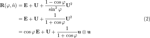
The last equation, which follows from U² = u⊗u − sin²φ E, is Eq. (3) of Ref. ^[4] after substitution of

$\frac{1-\cos\varphi}{\sin^2\varphi} =\frac{1-\cos\varphi}{1-\cos^2\varphi} = \frac{1}{1+\cos\varphi} .$

Indeed, write the rotation matrix in full, using the short-hand notations c = cos φ and h = (1-c)/(1-c²)

$\mathbf{R}(\varphi, \hat{n}) = \begin{pmatrix} c+hu_x^2 & h u_xu_y - u_z & h u_x u_z + u_y \\ h u_x u_y + u_z & c + h u_y^2 & h u_y u_z - u_x \\ h u_x u_z -u_y & h u_y u_z + u_x & c + h u_z^2 \\ \end{pmatrix},$

which is the matrix in Eq. (3) of Ref. ^[4]. If the vectors are parallel, f = t, then u = 0, U = 0 and f•t = cosφ = 1, so that the equation is well-defined—it gives R(φ, n) = E, as expected. Provided f and t are not anti-parallel, the matrix $\mathbf{R}(\varphi, \hat{n})$ can be computed easily and quickly. It requires not much more than the computation of the inner and cross product of f and t.

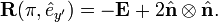
Case that "from" and "to" vectors are anti-parallel

If the vectors f and t are nearly anti-parallel, f ≈ − t, then f•t = cosφ ≈ − 1, and the denominator in Eq. (2) becomes zero, so that Eq. (2) is not applicable. The vector defining the rotation axis is nearly zero: u ≡ f × t ≈ f × (−f) ≈ 0.

Clearly, a two-fold rotation (angle 180°) around any rotation axis perpendicular to f will map f onto −f. This freedom in choice of the two-fold axis is consistent with the indeterminacy in the equation that occurs for cosφ = −1.

Since −E (inversion) sends f to −f, one could naively assume that all position vectors of the rigid body may be inverted by −E. However, if the rigid body is not symmetric under inversion (does not have a symmetry center), inversion turns the body into a non-equivalent one. For instance, if the body is a right-hand glove, inversion sends it into a left-hand glove; it is well-known that a right-hand and a left-hand glove are different.

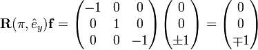
Recall that f is a unit vector. If f is on the z-axis, |f_z| = 1, then the following rotation around the y-axis turns f into −f:

$\mathbf{R}(\pi, \hat{e}_{y}) \mathbf{f} = \begin{pmatrix} -1 & 0 & 0 \\ 0 & 1 & 0 \\ 0 & 0 & -1 \\ \end{pmatrix} \begin{pmatrix} 0 \\ 0 \\\pm 1 \end{pmatrix} = \begin{pmatrix} 0 \\ 0 \\\mp 1 \end{pmatrix}$

If f is not on the z-axis, f_z ≠ 1, then the following orthogonal matrix sends f to −f and hence gives a 180° rotation of the rigid body

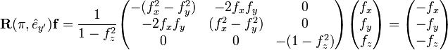
$\mathbf{R}(\pi, \hat{e}_{y'}) \mathbf{f} = \frac{1}{1-f^2_z} \begin{pmatrix} -(f^2_x-f^2_y) & -2f_xf_y & 0 \\ -2f_xf_y &(f^2_x-f^2_y) & 0 \\ 0 & 0 & -(1-f^2_z) \\ \end{pmatrix} \begin{pmatrix} f_x \\ f_y \\ f_z \end{pmatrix} = \begin{pmatrix} -f_x \\ -f_y \\ -f_z \end{pmatrix}$

To show this we insert

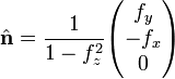
$\hat{\mathbf{n}} = \frac{1}{1-f^2_z} \begin{pmatrix} f_y \\-f_x \\0 \end{pmatrix}$

into the expression for rotation over 180° introduced earlier:

$\mathbf{R}(\pi, \hat{e}_{y'}) = -\mathbf{E} +2 \hat{\mathbf{n}}\otimes \hat{\mathbf{n}} .$

Note that the vector $\hat{\mathbf{n}}$ is normalized, because f is normalized, and that it lies in the x-y plane normal to the plane spanned by the z-axis and f; it is in fact a unit vector along a rotated y-axis obtained by rotation around the z-axis.

Given f = (f_x, f_y, f_z), the matrix $\mathbf{R}(\pi, \hat{e}_{y'})$ is easily and quickly calculated. The matrix rotates the body over 180° sending f to −f exactly. When −f and t are close, but not exactly equal, the earlier rotation formula Eq. (2), may be used to perform the final (small) rotation of the body that lets −f and t coincide exactly.

Change of rotation axis

Euler's theorem states that a rotation is characterized by a unique axis (an eigenvector with unit eigenvalue) and a unique angle. As a corollary of the theorem follows that the trace of a rotation matrix is equal to

$\mathrm{Tr}[\mathbf{R}(\varphi, \hat{n})] = 2\cos\varphi +1,$

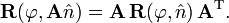
and hence the trace depends only on the rotation angle and is independent of the axis. Let A be an orthogonal 3×3 matrix (not equal to E), then, because cyclic permutation of matrices under the trace is allowed (i.e., leaves the trace invariant),

$\mathrm{Tr}[\mathbf{A} \mathbf{R}(\varphi, \hat{n}) \mathbf{A}^\mathrm{T}] = \mathrm{Tr}[ \mathbf{R}(\varphi, \hat{n}) \mathbf{A}^\mathrm{T}\mathbf{A}] = \mathrm{Tr}[\mathbf{R}(\varphi, \hat{n})] .$

As a consequence it follows that the two matrices

$\mathbf{R}(\varphi, \hat{n})\quad \hbox{and}\quad \mathbf{A} \mathbf{R}(\varphi, \hat{n}) \mathbf{A}^\mathrm{T}$

describe a rotation over the same angle φ but around different axes. The eigenvalue equation can be transformed

$\mathbf{R}(\varphi, \hat{n})\;\hat{n} = \hat{n} \;\Longrightarrow\; \left(\mathbf{A}\,\mathbf{R}(\varphi, \hat{n})\,\mathbf{A}^\mathrm{T}\right) \;\mathbf{A}\hat{n} = \mathbf{A}\hat{n}$

which shows that the transformed eigenvector is the rotation axis of the transformed matrix, or

$\mathbf{R}(\varphi, \mathbf{A}\hat{n})= \mathbf{A}\,\mathbf{R}(\varphi, \hat{n})\,\mathbf{A}^\mathrm{T} .$

References

↑ L. C. Biedenharn and J. D. Louck, Angular Momentum in Quantum Physics, Addison-Wesley, Reading, Mass. (1981) ISBN 0-201-13507-8
↑ Wikipedia Retrieved July 20, 2009
↑ E. T. Whittaker, A Treatise on the Dynamics of Particles and Rigid Bodies, Cambridge University Press (1965)
↑ ^4.0 ^4.1 T. Möller and J. F. Hughes, J. Graphics Tools, 4 pp. 1–4 (1999).

[0] L. C. Biedenharn and J. D. Louck, Angular Momentum in Quantum Physics, Addison-Wesley, Reading, Mass. (1981) ISBN 0-201-13507-8

[1] Wikipedia Retrieved July 20, 2009

[2] E. T. Whittaker, A Treatise on the Dynamics of Particles and Rigid Bodies, Cambridge University Press (1965)

[MH-3] 4.0 ^4.1 T. Möller and J. F. Hughes, J. Graphics Tools, 4 pp. 1–4 (1999).

[1]

[2]

[3]

[4]

Rotation matrix

Contents

Connection of an orthogonal matrix to a rotation

Properties of an orthogonal matrix

Compact notation

Explicit expression of rotation operator

Explicit expression of rotation matrix

Vector rotation

Case that "from" and "to" vectors are anti-parallel

Change of rotation axis

References

Personal tools

Namespaces

Variants

Views

Actions

Search

Navigation

Community

Toolbox